Quantitative Credit Portfolio Management

Practical Innovations for Measuring and Controlling Liquidity, Spread, and Issuer Concentration Risk

Arik Ben Dor, Lev Dynkin, Jay Hyman, Bruce D. Phelps

• Publisher: Wiley
• Year: 2011
• Print ISBN: 9781118117699
• eBook ISBN: 9781118167427
• Edition: 1
• Topic: Business
• Subtopic: Investimenti e titoli
• Index: Business

An innovative approach to post-crash credit portfolio management

Credit portfolio managers traditionally rely on fundamental research for decisions on issuer selection and sector rotation. Quantitative researchers tend to use more mathematical techniques for pricing models and to quantify credit risk and relative value. The information found here bridges these two approaches. In an intuitive and readable style, this book illustrates how quantitative techniques can help address specific questions facing today's credit managers and risk analysts.

A targeted volume in the area of credit, this reliable resource contains some of the most recent and original research in this field, which addresses among other things important questions raised by the credit crisis of 2008-2009. Divided into two comprehensive parts, Quantitative Credit Portfolio Management offers essential insights into understanding the risks of corporate bonds—spread, liquidity, and Treasury yield curve risk—as well as managing corporate bond portfolios.

• Presents comprehensive coverage of everything from duration time spread and liquidity cost scores to capturing the credit spread premium
• Written by the number one ranked quantitative research group for four consecutive years by Institutional Investor
• Provides practical answers to difficult question, including: What diversification guidelines should you adopt to protect portfolios from issuer-specific risk? Are you well-advised to sell securities downgraded below investment grade?

Credit portfolio management continues to evolve, but with this book as your guide, you can gain a solid understanding of how to manage complex portfolios under dynamic events.

PART ONE

Measuring the Market Risks of Corporate Bonds

CHAPTER 1

Measuring Spread Sensitivity of Corporate Bonds

Duration Times Spread (DTS)

The standard presentation of the asset allocation in a portfolio or a benchmark is in terms of percentage of market value. It is widely recognized that this is not sufficient for fixed income portfolios, where differences in duration can cause two portfolios with the same allocation of market weights to have extremely different exposures to macro-level risks. A common approach to structuring a portfolio or comparing it to a benchmark is to partition it in homogeneous market cells comprised of securities with similar characteristics. Many fixed income portfolio managers have become accustomed to expressing their cell allocations in terms of contributions to duration—the product of the percentage of portfolio market value represented by a given market cell and the average duration of securities comprising that cell. This represents the sensitivity of the portfolio to a parallel shift in yields across all securities within this market cell. For credit portfolios, the corresponding measure would be contributions to spread duration, measuring the sensitivity to a parallel shift in spreads. Determining the set of active spread duration bets from different market cells and issuers is one of the primary decisions taken by credit portfolio managers.

Yet all spread durations were not created equal. Just as one could create a portfolio that matches the benchmark exactly by market weights, but clearly takes more credit risk (e.g., by investing in the longest duration credits within each cell), one could match the benchmark exactly by spread duration contributions and still take more credit risk—by choosing the securities with the widest spreads within each cell. These bonds presumably trade wider than their peer groups for a reason—that is, the market consensus has determined that they are more risky—and are often referred to as high beta, because their spreads tend to react more strongly than the rest of the market to a systematic shock. Portfolio managers are well aware of this, but many tend to treat it as a secondary issue rather than as an intrinsic part of the allocation process.

To reflect the view that higher spread credits represent greater exposures to systematic risks, we introduce a new risk sensitivity measure that utilizes spreads as a fundamental part of the credit portfolio management process. We represent sector exposures by contributions to duration times spread (DTS), computed as the product of market weight, spread duration, and spread. For example, an overweight of 5% to a market cell implemented by purchasing bonds with a spread of 80 basis points (bps) and spread duration of three years would be equivalent to an overweight of 3% using bonds with an average spread of 50 bps and spread duration of eight years.

To understand the intuition behind this new measure, consider the return, Rspread, due strictly to change in spread. Let D denote the spread duration of a bond and s its spread; the spread change return is then:1

(1.1)

Or, equivalently,

(1.2)

That is, just as spread duration is the sensitivity to an absolute change in spread (e.g., spreads widen by 5 bps), DTS

is the sensitivity to a relative change in spread. Note that this notion of relative spread change provides for a formal expression of the idea mentioned earlier—that credits with wider spreads are riskier since they tend to experience greater spread changes.

In the absolute spread change approach shown in equation (1.1), we can see that the volatility of excess returns can be approximated by

(1.3)

while in the relative spread change approach of equation (1.2), excess return volatility follows

(1.4)

Given that the two representations above are equivalent, why should one of them be preferable to another?

In this chapter, we provide ample evidence that the advantage of the second approach, based on relative spread changes, is due to the stability of the associated volatility estimates. Using a large sample with over 560,000 observations spanning the period of September 1989 to January 2005, we demonstrate that the volatility of spread changes (both systematic and idiosyncratic) is linearly proportional to spread level.2 This relation holds for both investment-grade and high-yield credit irrespective of the sector, duration, or time period. Furthermore, these results are not confined to the realm of U.S. corporate bonds, but also extend to other spread asset classes with a significant default risk. The next two chapters, for example, contain similar results for credit default swaps, European corporate and sovereign bonds, and emerging market sovereign debt denominated in U.S. dollars. Indeed, as we show in Chapter 4, even from a theoretical standpoint, structural credit risk models such as Merton (1974) imply a near-linear relationship between spread level and volatility. This explains why relative spread volatilities of spread asset classes are much more stable than absolute spread volatilities, both across different sectors and credit quality tiers, and also over time. In Chapter 10, we present more recent empirical evidence showing the benefits of using DTS during the 2007–2009 credit crisis.

The paradigm shift we advocate has many implications for portfolio managers, both in terms of the way they manage exposures to industry and quality factors (systematic risk) and in terms of their approach to issuer exposures (non-systematic risk). Throughout the chapter, we present evidence that the relative spread change approach offers increased insight into both of these sources of risk. Furthermore, in Chapter 5, we also show that DTS is an important determinant of corporate bond liquidity.

ANALYSIS OF CORPORATE BOND SPREAD BEHAVIOR

How should the risk associated with a particular market sector be measured? Typically, for lack of any better estimator, the historical return volatility of a particular sector over some prior time period is used to forecast its volatility for the coming period.3 For this approach to be reliable, these volatilities have to be fairly stable. Unfortunately, this is not always the case.

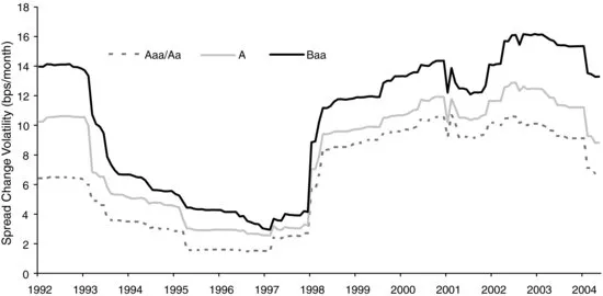
As an example, Figure 1.1 shows the 36-month trailing volatility of spread changes for various credit ratings comprising the U.S. Corporate Index between September 1989 and January 2005. It is clear from the chart that spread volatility decreased substantially until 1998 and then increased significantly from 1998 through 2005. The dramatic rise in spread volatility since 1998 was only a partial response to the Russian Crisis and the Long-Term Capital Management debacle as volatility did not revert to its pre-1998 level.

FIGURE 1.1 Spread Change Volatility by Credit Rating (trailing 36 months; September 1989–January 2005)

Source: Barclays Capital.

FIGURE 1.2 Spread Change Volatility by Spread Range (trailing 36 months; September 1989–January 2005)

Source: Barclays Capital.

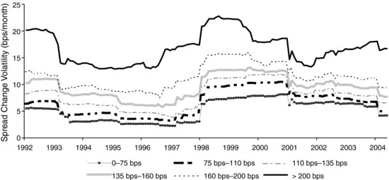
If the investment-grade corporate universe is partitioned by spread levels, we find that the volatilities of the resulting spread buckets are considerably more stable, as seen in Figure 1.2. After an initial shock in 1998, the volatilities within each spread bucket revert almost exactly to their pre-1998 level (beginning in August 2001, exactly 36 months after the Russian crisis occurred). In this respect, one could relate the results of Figure 1.1 to an increase in spreads—both across the market and within each quality group.

FIGURE 1.3 Absolute and Relative Spread Change Volatility of Baa-Rated Bonds (trailing 36 months)

Source: Barclays Capital.

As suggested by equation (1.4), a potential remedy to the volatility instability problem is to approximate the absolute spread volatility (bps/month) by multiplying the historically observed relative spread volatility (%/month) by the current spread (bps). This improves the estimate if relative spread volatility is more stable than absolute spread volatility. The results in Figure 1.2 point in this direction and indicate a relationship between spread level and volatility.

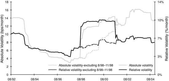
Figure 1.3 plots side-by-side the volatility of absolute and relative spread changes of the Corporate Baa index (relative spread changes are calculated simply as the ratio of spread change to the beginning of month spread level). The comparison illustrates that a modest stability advantage is gained ...

Table of contents

• Cover
• Endorsements
• Series
• Title Page
• Copyright
• Dedication
• Acknowledgments
• Foreword
• Introduction
• Notes on Terminology
• PART ONE: Measuring the Market Risks of Corporate Bonds
• PART TWO: Managing Corporate Bond Portfolios
• References
• Index