Fundamentals of Digital Image Processing

A Practical Approach with Examples in Matlab

Chris Solomon, Toby Breckon

• Publisher: Wiley
• Year: 2011
• Print ISBN: 9780470844731, 9780470844724
• eBook ISBN: 9781119957003
• Edition: 1
• Topic: Physical Sciences
• Subtopic: Physics
• Index: Physics

This is an introductory to intermediate level text on the science of image processing, which employs the Matlab programming language to illustrate some of the elementary, key concepts in modern image processing and pattern recognition. The approach taken is essentially practical and the book offers a framework within which the concepts can be understood by a series of well chosen examples, exercises and computer experiments, drawing on specific examples from within science, medicine and engineering.

Clearly divided into eleven distinct chapters, the book begins with a fast-start introduction to image processing to enhance the accessibility of later topics. Subsequent chapters offer increasingly advanced discussion of topics involving more challenging concepts, with the final chapter looking at the application of automated image classification (with Matlab examples).

Matlab is frequently used in the book as a tool for demonstrations, conducting experiments and for solving problems, as it is both ideally suited to this role and is widely available. Prior experience of Matlab is not required and those without access to Matlab can still benefit from the independent presentation of topics and numerous examples.

• Features a companion website www.wiley.com/go/solomon/fundamentals containing a Matlab fast-start primer, further exercises, examples, instructor resources and accessibility to all files corresponding to the examples and exercises within the book itself.
• Includes numerous examples, graded exercises and computer experiments to support both students and instructors alike.

1
Representation

In this chapter we discuss the representation of images, covering basic notation and information about images together with a discussion of standard image types and image formats. We end with a practical section, introducing Matlab’s facilities for reading, writing, querying, converting and displaying images of different image types and formats.

1.1 What is an image?

A digital image can be considered as a discrete representation of data possessing both spatial (layout) and intensity (colour) information. As we shall see in Chapter 5, we can also consider treating an image as a multidimensional signal.

1.1.1 Image layout

The two-dimensional (2-D) discrete, digital image I(m, n) represents the response of some sensor (or simply a value of some interest) at a series of fixed positions (m = 1,2,. .., M; n = 1,2,. .., N) in 2-D Cartesian coordinates and is derived from the 2-D continuous spatial signal I(x, y) through a sampling process frequently referred to as discretization. Discretization occurs naturally with certain types of imaging sensor (such as CCD cameras) and basically effects a local averaging of the continuous signal over some small (typically square) region in the receiving domain.

The indices m and n respectively designate the rows and columns of the image. The individual picture elements or pixels of the image are thus referred to by their 2-D (m, n) index. Following the Matlab^® convention, I(m, n) denotes the response of the pixel located at the mth row and nth column starting from a top-left image origin (see Figure 1.1). In other imaging systems, a column-row convention may be used and the image origin in use may also vary.

Although the images we consider in this book will be discrete, it is often theoretically convenient to treat an image as a continuous spatial signal: I(x, y). In particular, this sometimes allows us to make more natural use of the powerful techniques of integral and differential calculus to understand properties of images and to effectively manipulate and process them. Mathematical analysis of discrete images generally leads to a linear algebraic formulation which is better in some instances.

Figure 1.1 The 2-D Cartesian coordinate space of an M × N digital image

The individual pixel values in most images do actually correspond to some physical response in real 2-D space (e.g. the optical intensity received at the image plane of a camera or the ultrasound intensity at a transceiver). However, we are also free to consider images in abstract spaces where the coordinates correspond to something other than physical space and we may also extend the notion of an image to three or more dimensions. For example, medical imaging applications sometimes consider full three-dimensional (3-D) reconstruction of internal organs and a time sequence of such images (such as a beating heart) can be treated (if we wish) as a single four-dimensional (4-D) image in which three coordinates are spatial and the other corresponds to time. When we consider 3-D imaging we are often discussing spatial volumes represented by the image. In this instance, such 3-D pixels are denoted as voxels (volumetric pixels) representing the smallest spatial location in the 3-D volume as opposed to the conventional 2-D image.

Throughout this book we will usually consider 2-D digital images, but much of our discussion will be relevant to images in higher dimensions.

1.1.2 Image colour

An image contains one or more colour channels that define the intensity or colour at a particular pixel location I(m, n).

In the simplest case, each pixel location only contains a single numerical value representing the signal level at that point in the image. The conversion from this set of numbers to an actual (displayed) image is achieved through a colour map. A colour map assigns a specific shade of colour to each numerical level in the image to give a visual representation of the data. The most common colour map is the greyscale, which assigns all shades of grey from black (zero) to white (maximum) according to the signal level. The greyscale is particularly well suited to intensity images, namely images which express only the intensity of the signal as a single value at each point in the region.

Figure 1.2 Example of grayscale (left) and false colour (right) image display (See colour plate section for colour version)

In certain instances, it can be better to display intensity images using a false-colour map. One of the main motives behind the use of false-colour display rests on the fact that the human visual system is only sensitive to approximately 40 shades of grey in the range from black to white, whereas our sensitivity to colour is much finer. False colour can also serve to accentuate or delineate certain features or structures, making them easier to identify for the human observer. This approach is often taken in medical and astronomical images.

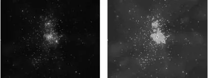
Figure 1.2 shows an astronomical intensity image displayed using both greyscale and a particular false-colour map. In this example the jet colour map (as defined in Matlab) has been used to highlight the structure and finer detail of the image to the human viewer using a linear colour scale ranging from dark blue (low intensity values) to dark red (high intensity values). The definition of colour maps, i.e. assigning colours to numerical values, can be done in any way which the user finds meaningful or useful. Although the mapping between the numerical intensity value and the colour or greyscale shade is typically linear, there are situations in which a nonlinear mapping between them is more appropriate. Such nonlinear mappings are discussed in Chapter 4.

In addition to greyscale images where we have a single numerical value at each pixel location, we also have true colour images where the full spectrum of colours can be represented as a triplet vector, typically the (R,G,B) components at each pixel location. Here, the colour is represented as a linear combination of the basis colours or values and the image may be considered as consis...

Table of contents

• Cover
• Title Page
• Copyright
• Preface
• Using the book website
• 1: Representation
• 2: Formation
• 3: Pixels
• 4: Enhancement
• 5: Fourier transforms and frequency-domain processing
• 6: Image restoration
• 7: Geometry
• 8: Morphological processing
• 9: Features
• 10: Image Segmentation
• 11 Classification
• Further reading
• Index