Finite Element Simulation of Heat Transfer

Jean-Michel Bergheau, Roland Fortunier

• Publisher: Wiley-ISTE
• Year: 2013
• Print ISBN: 9781848210530
• eBook ISBN: 9781118623428
• Edition: 1
• Topic: Physical Sciences
• Subtopic: Thermodynamics

This book introduces the finite element method applied to the resolution of industrial heat transfer problems. Starting from steady conduction, the method is gradually extended to transient regimes, to traditional non-linearities, and to convective phenomena. Coupled problems involving heat transfer are then presented. Three types of couplings are discussed: coupling through boundary conditions (such as radiative heat transfer in cavities), addition of state variables (such as metallurgical phase change), and coupling through partial differential equations (such as electrical phenomena). A review of the various thermal phenomena is drawn up, which an engineer can simulate. The methods presented will enable the reader to achieve optimal use from finite element software and also to develop new applications.

PART 1

Steady State Conduction

Introduction

In this part we introduce the finite element method in the simplest field of thermal science: steady state conduction. We therefore consider a solid Ω undergoing thermal loads and try to determine the temperature field

in this solid, when it is in equilibrium with the external environment. In this part, it is assumed that no quantity involved depends on time. Thermal loads are therefore constant and the solid is motionless. The equilibrium state sought corresponds to a steady state. Besides, we will restrict our study to the linear case in which the mathematical field is clearly identified. The finite element method is introduced according to the following three steps.

Firstly, the physical problem to solve is analyzed from a mathematical point of view. This leads to a series of three problems (equations [1.8], [1.10] and [1.13]). Problem [1.8] is a partial differential equation resulting directly from physical modeling with its boundary conditions. Problem [1.10] turns this partial differential equation into a variational equation by means of the weighted residual method. Finally, problem [1.13], often called weak form, is the basis of the finite element method.

It is possible to find an approximate solution to each of the three problems [1.8], [1.10] and [1.13]. For this purpose, several methods are used. Each of them will be illustrated by a work example: an induction-heated plate. We will use a physical model to describe this example, then seek approximate solutions (the temperature field) of problems [1.8], [1.10] and [1.13] related to this physical model.

Chapter 2 deals with the finite element method. This method is based upon the weak form described in Chapter 1. The approximation used is called finite element approximation. It consists of discretizing the geometry (the mesh) and approximating the temperatures sought (nodal approximation). This step makes it possible to write the problem to solve in a discretized form, which is very appropriate for a computer numerical solution. In this chapter, the various steps of the finite element method will be illustrated by a new work example: thermal conduction in a plate with holes.

In Chapter 3, we introduce isoparametric finite elements starting from the notion of the reference element. This makes it possible to develop simple and rapid methods for the calculation of the element quantities involved in the discrete problem formulation. The major types of isoparametric elements are also described in detail in this chapter.

Chapter 1

Problem Formulation

1.1. Physical modeling

In this chapter we describe the different steps of physical modeling leading in the next section to a boundary value problem. These steps are:

1) writing the equation expressing the solid thermal equilibrium,

2) introducing the Fourier law connecting the heat flux to the temperature gradient,

3) formulating boundary conditions.

1.1.1. Thermal equilibrium equation

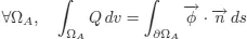
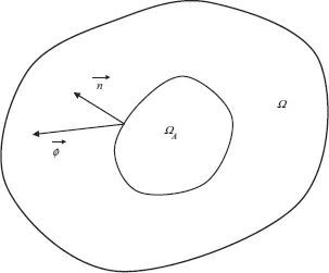
Figure 1.1 illustrates a homogenous solid Ω. In order to write that this solid is in thermal equilibrium, consider any portion Ω_A related to this solid and write that the heat produced on that portion is equal to the heat flux coming out of it, i.e.:

[1.1]

In this equation,

is a vector characterizing the heat flux surface density (in W/m²) coming out of Ω_A through its boundary ∂Ω_A,

is the outward unit normal to this surface, and Q is a scalar representing an internal heat volumetric source (in W/m³) in Ω_A. Among the physical phenomena represented by this volumetric term, we can include Joule effect heating (conduction or induction), heat dissipation by plastic deformation, etc.

Figure 1.1. Solid thermal equilibrium

If the divergence theorem is now applied (integration by ...

Table of contents

• Cover
• Title Page
• Copyright
• Introduction
• PART 1: Steady State Conduction
• PART 2: Transient State, Non-linearities, Transport Phenomena
• PART 3: Coupled Phenomena
• Bibliography
• Index