![]()
Section F: HDR Image Processing
31
HDR Pixel and Spatial Algorithms
31.1 Topics
In Section F we will describe and analyze HDR algorithms that we have divided into a number of categories. We will emphasize the many variants of Retinex and ACE image processing and review analytical interpretations. We describe a number of different techniques to evaluate the success of different algorithms. Finally, we use what we have learned to discuss future research in HDR imaging.
31.2 Introduction – HDR Image Processing Algorithms
In Section A we described how the ideas of silver halide photography have influenced our thinking about images. We may never be sure if analyzing images one pixel at a time comes from Euclidean geometry, or the chemical mechanisms of silver halide photography, or the later influence of Thomas Young’s tricolor hypothesis. It may be a combination of all three. Regardless, there are many useful systems that perform successful predictions with calculations that limit the input information to that of a single pixel. Silver halide film models and colorimetry are good examples. We can calculate the response of a film from the quanta catch of the silver-halide grains at a small local region of the film. The film’s response to quanta catch is the same everywhere in the image. As well, we can predict whether two different spectra (wavelength vs. energy distributions) will match to humans. As we have seen many times in this text, calculations that are restricted to the information from a single pixel cannot predict human appearance, and are of limited value in HDR imaging.
Our analysis has the goal of evaluating an algorithm’s ability to render all types of scenes. If the process mimics the human visual system, then it must render appropriately LDR, HDR, low-average and high-average scenes using the same algorithm parameters. Using this as a performance standard is very helpful in evaluating the great variety of algorithms.
We will review image processing algorithms that use light (quanta catch) from:
one pixel,
a local group of pixels,
all the pixels,
and all the pixels in a way that mimics vision.
31.3 One Pixel – Tone Scale Curves
It is easy and efficient to apply tone scale curves to digital images. While color negative-to-print technology installed a fixed tone scale in the factory, digital photography can apply it using the individual’s personal computer. Although the practice is completely different, the principles are the same. Jones and colleagues sought the best compromise for optimal rendition of all types of scenes. They measured the limits of veiling glare, and designed negatives that in single exposures captured all the dynamic range possible after glare (Section B). There is no fundamental difference between film and digital tone-scale rendering. Both cannot address the issue raised by Land’s Black and White Mondrian, and “John at Yosemite” experiments. Nonuniform illumination, sun and shade, puts the same light on the camera’s film plane from white areas in the shade, and black areas in the sun. HDR scene rendition that mimics human vision requires spatial image processing.
There is a great irony in using Tone Scales to improve digital imaging. Tone scales were built into the chemistry of film processing. A great deal of practical image-quality research on the scenes people photographed determined the optimal tone scale response for prints and transparencies (Mees, 1961; Mees & James, 1966). Tone scales for film photography were optimal for pixel based image processing of all scenes. Pixel-based processing had to be the best compromise. It cannot respond differently to scene content. However, digital imaging has made spatial processing possible. Unlike film, that restricted spatial interactions to a few microns, electronic imaging has freed us from the fixed compromise of a global tone scale.
31.3.1 One Pixel – Histogram
A popular tool among digital photographers is histogram equalization. Histograms that plot the number of pixels for all camera quantization levels (e.g., 0 to 255) are very helpful in evaluating camera exposures. Over- and under-exposure is easily recognized in histogram plots. Engineers have developed programs that group quantization levels into bins, and then redistribute the bins with the goal of having a more uniform distribution of digital values. Histogram equalization programs process the image using the pixel-value population. It assumes that the image will look better if all the bins have an equal count. Histograms equalization programs completely ignore the spatial information in the input, and significantly distort the spatial relationships in the output. Many scenes are harmed by histogram-equalization renditions because they change the spatial relationships of image content.
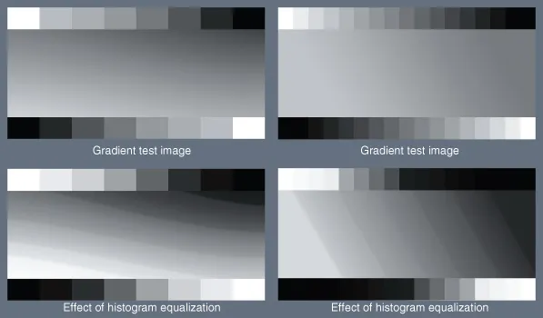
Figure 31.1 shows the effects of histogram equalization on a pair of test targets made up of gradients and uniform gray squares. The left and right targets have the same maximum, minimum and range. They have different gradients in the middle and more gray steps between max and min on the right. They differ in the image statistics; the number of pixels per digital value (0 to 255). In the gradients, pixels have very similar values to nearby pixels. Since histogram equalization just evaluates the statistics of the image, it does not preserve subtle local relationships. In the pair of test targets the gradient appears smooth and low in contrast. In the pair of histogram-equalized images below, the gradients are broken up into different bands of luminance, showing the algorithm’s indifference to local relationships. Furthermore, the gray scales at top and bottom have been rendered with lower contrast near white and black, but with higher contrast for mid-grays.
Humans do not use image statistics in generating appearances. As we have seen in Sections D and E, the spatial relationships of the image content control appearances.
31.3.2 One Pixel – LookUp Tables
There is a great advantage to single-pixel processing. It is fast, low-cost, and requires minimal hardware. HDR algorithms frequently use LookUp Tables (LUTs) because they require only a small number of memory locations per color to load the digital values of the output. The operation is to read the memory value out at the appropriate address. This operation is simpler and faster than multiplying two numbers.
Single pixel techniques are ideal for manipulating the appearance of individual images which have a particular problem. There are many HDR guide books that can help to solve particular problems for particular scenes using multiple digital exposures, RAW format cameras and LUTs (Bloch, 2007; Freeman, 2008; McCollough, 2008; Correll, 2009; Fraser & Schewe, 2009). Although they often use the less powerful three 1-D LUT approach, they do great things to individual images.
Three-dimensional LUTs are an extremely powerful tool in making accurate reproductions and controlling color profiles (Pugsley, 1975; Kotera et al., 1978 Abdulwahab et al., 1989, McCann, 1995; 1997). Recall the analogy of color reproduction as the act of moving from an old house to a new one with different size rooms. The 3-D LUT process lets one use a different strategy in each room. It is much more powerful than three 1-D LUTs. Such 3-D LUTs play a major role in the color calibration processes of digital printers, displays and color management systems (Green, 2010).
31.3.3 Using 1-D LookUp Tables for Rendering HDR Scene Captures
Kate Devlin (2002) and Carlo Gatta (2006) wrote extensive reviews of the many tone scale LUTs and their underlying principles. Reinhard et al. (2006, Chapter 6) review the digital versions of conventional film tone-scale techniques. Although Reinhard provides many color illustrations of the processes, it is difficult to compare these approaches because each of the examples uses a different test image.
Applying the same pixel processing LUT (global operators) to any, and all, scene reproductions is not realistic. Some algorithms use a two step process to incorporate models of human vision. First, they assume that multiple-exposures can measure accurate scene luminance. Second, they apply a global-tone-scale map derived from psychometric functions, measured using isolated spots of light, rather than using scenes.
Many algorithms use some kind of psychophysical data to convert scene radiance to visual appearance. As well, psychophysical data are sometimes used outside of their original context. Similarities with human vision are taken as an inspiration, rather than modeling calibrated scene input with precise implementation of the experimental data. They have been inspired by Steven’s data on brightness perception (Tumblin & Rushmeier, 1993), Blackwell contrast sensitivity model (Ward, 1994), models of photopic and scotopic adaptation (Ferwerda, et al., 1996) differential nature of visual sensation (Larson et al., 1997), image statistics (Holm, 1996) adaptation and gaze (Scheel et al., 2000). Reinhard and Devlin (2004) used physiological data to modify uncalibrated cameras’ scene capture. They used Hood’s modification of Naka & Rushton’s famous equation describing an electrode’s extra-cellular post-receptor graded S-potential response of excised fish retinas.
There are many problems with such algorithms that prevent them from accurately predicting human vision. The captured scene data is an ...