![]()
PART I
Introductory Theories
![]()
CHAPTER I
FUNCTIONAL DETERMINANTS AND MATRICES
1.Geometrical terminology.
In analytical geometry it frequently happens that complicated algebraic relationships represent simple geometrical properties. In some of these cases, while the algebraic relationships are not easily expressed in words, the use of geometrical language, on the contrary, makes it possible to express the equivalent geometrical relationships clearly, concisely, and intuitively. Further, geometrical relationships are often easier to discover than are the corresponding analytical properties, so that geometrical terminology offers not only an illuminating means of exposition, but also a powerful instrument of research. We can therefore anticipate that in various questions of analysis it will be advantageous to adopt terms taken over from geometry.
For this purpose it is essential to adopt the fundamental convention of using the term point of an abstract n-dimensional manifold (n being any positive integer whatever) to denote a set of n values assigned to any n variables x1, x2, … xn. This is an obvious extension of the use of the term in the one-to-one correspondence which can be established between pairs or triplets of co-ordinates and the points of a plane or space, for the cases n = 2 and n = 3 respectively. For the case of n variables we can thus also speak of a field of points (rather than of values assigned to the x’s), and of the region round a specified point xi (i = 1, 2, … n).
If the x’s are n functions xi(t) of a real variable t, then when t varies continuously between t0 and t1 we get a simply infinite succession of points, the aggregate of which (as for n = 2 and n = 3) is called a line, and more precisely an arc or segment of a line.
2.Functional determinants and change of variables.
Let there be n functions of n variables:
ui(x1, x2, … xn),
the functions and their derivatives to any required degree being supposed finite and continuous in the field considered.
To simplify the notation, let x (without a suffix) represent not only (as is usual) any one of the n variables x1, x2, … xn, but also (as is sometimes done) the whole set of them; and similarly for other letters which will be used farther on. With this convention the given functions can be written in the abridged form:
ui(x).
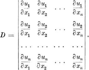
With the usual notation, the functional determinant or Jacobian of the u’s is the determinant of the nth order whose terms are the first derivatives of the u’s; i.e.
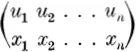
Such a determinant is sometimes represented by the abridged notation
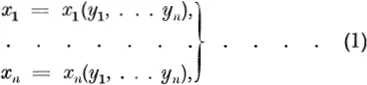
analogous to that used for fractions and substitutions, the set of functions u representing the numerator and the set of variables x the denominator of a fraction. The analogy of form is justified by the analogy of properties, as can be seen by considering the effect on a functional determinant of a change of variables. For let the x’s be functions of n variables y,
and suppose further that these equations represent a reversible transformation, i.e. that they also define the y’s as functions of the x’s, or, in other words, that they are soluble with respect to the y’s. If then the u’s are considered as functions of the y’s (being given in terms of the x’s, which are functions of the y’s), and the corresponding functional determinant
is formed, it will be found, as will be shown below in § 4, that D1 = D multiplied b...