![]()
Chapter 1
MATRICES: BASIC SKILLS AND APPLICATIONS
1.1 Definitions, Addition, Scalar Multiplication, and Notation
Arithmetic is the study of numbers. Geometry is the study of shapes. Algebra is the study of equations. And linear algebra, the subject matter of the first four chapters of this book, is the study of matrices.
1.1.1 Definition
A matrix (plural: matrices) is a rectangular array of numbers.
1.1.2 Example
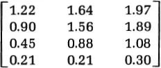
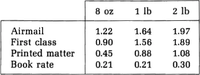
is a matrix. You have already seen matrices in many contexts. The matrix above, for example, appears in a table of the cost of mailing books:
The first chapter of this text reminds you of some facts you already know about matrices, introduces some unfamiliar applications, and explores some properties of matrices that mathematicians use. In many ways matrices are like numbers; they can be added and multiplied, for example. And they also have novel useful properties, as we shall see. The next three chapters explore these properties further.
In Chapters 5 through 8 of this book rectangular arrays of numbers will be used in a somewhat different subject, linear programming, which uses some of the same skills that you will develop in linear algebra. Linear programming problems involve maximizing or minimizing some variable (often profit or cost, respectively) given certain restrictions on other variables. A good course in first-year algebra is the only prerequisite for this text; if you need to review algebra, you can read the appendixes and do the exercises given there. No geometry or calculus will be used.
The words row and column in matrix theory follow ordinary English usage. The elements (numbers) in the first row of the matrix in Example 1.1.2 are 1.22, 1.64, and 1.97; the elements in the first column are 1.22, 0. 90, 0.45, and 0.21. We say that this matrix is a 4 by 3 matrix because it has 4 rows and 3 columns.
1.1.3 Definition
A matrix with n rows and m columns is said to be of dimension n by m.
1.1.4 Definition
Two matrices are said to be equal if they have the same dimension and each element in one is equal to the corresponding element in the other.
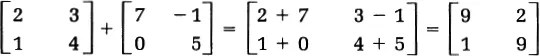
Matrix addition is straightforward. Two matrices must have the same dimension if they are to be added; to add them, we merely add corresponding elements.
1.1.5 Example
1.1.6 Example
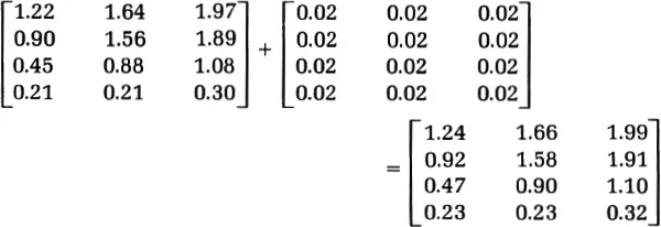
Suppose that the Postal Service decides to increase the rates across-the-board by $0.02 over the rates given in Example 1.1.2. To find the new matrix describing the postal rates, we add to our original matrix one that has the same dimensions and in which each element equals 0.02.
Subtraction of matrices is similar to addition; it is done element by element. Again, the matrices must have the same dimension.
1.1.7 Example
If the Postal Service decides to decrease (!) the rates across-the-board by $0.02 from those given in Example 1.1.2, we can find the new rates as follows:
Suppose that the Postal Service decides instead to increase all the rates by 10 percent. This would be the same as multiplying all the rates by 1.1 (because an increase of 10 percent is the same as adding 0.1 times the original price to the original price and 0.1x + x = 1.1x). Thus, to get the matrix describing the new rates, we would use scalar multiplication; that is, we would multiply every element of the matrix by the same number (which is called a “scalar” in this context).
1.1.8 Example
Use scalar multiplication to show how a 10 percent rate increase affects the postal rate matrix of Example 1.1.2. Round off the results to the nearest cent.
If the postal rates are doubled, the scalar multiplication of the matrix is easy indeed:
Matrix Notation
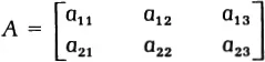
Often we shall want to denote the elements of a matrix symbolically. The standard way of writing a general 2 by 3 matrix is
The subscripts look like two-digit numbers occurring in the expected order, but each subscript actually consists of two different one-digit numbers, the first indicating the row in which the element appears and the second indicating the column. The upper ri...