Essential Demographic Methods

Kenneth W. Wachter

• Publisher: Harvard University Press
• Year: 2014
• ISBN:
  9780674369764
• Topic: Social Sciences
• Subtopic: Demography
• Index: Social Sciences

Essential Demographic Methods brings to readers the full range of ideas and skills of demographic analysis that lie at the core of social sciences and public health. Classroom tested over many years, filled with fresh data and examples, this approachable text is tailored to the needs of beginners, advanced students, and researchers alike. An award-winning teacher and eminent demographer, Kenneth Wachter uses themes from the individual lifecourse, history, and global change to convey the meaning of concepts such as exponential growth, cohorts and periods, lifetables, population projection, proportional hazards, parity, marity, migration flows, and stable populations. The presentation is carefully paced and accessible to readers with knowledge of high-school algebra. Each chapter contains original problem sets and worked examples.From the most basic concepts and measures to developments in spatial demography and hazard modeling at the research frontier, Essential Demographic Methods brings out the wider appeal of demography in its connections across the sciences and humanities. It is a lively, compact guide for understanding quantitative population analysis in the social and biological world.

1

Exponential Growth

1.1 The Balancing Equation

The most basic demographic equation is the “Balancing Equation”. The Balancing Equation for the world as a whole from 2010 to 2011 takes the form

Here, K(2010) is the world population at the start of 2010, B(2010) are the births during 2010, D(2010) are the deaths during 2010, and K(2011) is the population at the start of 2011. The letter “K” is traditionally used for population instead of “P”, to avoid confusion with probability, which also starts with p. Estimated values for the numbers that go into the balancing equation for 2010 are shown in Table 1.1. Sources for this table and later tables are listed with abbreviations found in Appendix A.

The world population is a “closed population”. The only way to enter is by being born. The only way to exit is by dying. The general form of the Balancing Equation for a closed population is

As before, K(t) is the size of the population at time t, n is the length of a period like 1 year or 10 years, and B(t) and D(t) are the births and deaths during the period from t to t + n.

Table 1.1 The world population 2010 to 2011

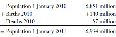
Source: Population Data Sheet of the Population

Reference Bureau (PRB) for 2010.

The Balancing Equation for national or regional populations is more complicated, because such populations also change through migration. The U.S. Census Bureau keeps track of the nation’s population by age, sex, and race from decade to decade with a refinement of the Balancing Equation called “Demographic Analysis” with a capital “D” and capital “A”. The Bureau’s Balancing Equation includes several kinds of migration. In much of this book, however, we shall be studying models for closed populations. This is a simplification that help us to understand basic concepts more easily. But no one should imagine that most national or local populations are at all close to being closed.

World population reached 7 billion during 2011. Seven billion, in American English, is seven thousand million. It is written with a 7 followed by nine zeros, or 7 ∗ 10⁹. Computers have popularized words for large numbers based on Greek prefixes: kilo for thousands (10³), mega for millions (10⁶), giga for billions (10⁹), and tera for trillions (10¹²). Going further, we have peta for 10¹⁵, exa for 10¹⁸, and zetta for 10²¹. In this terminology, the world contains 7 gigapersons.

Large numbers like these are needed when we study global resources and the impact of humans on the environment of our planet. For instance, the total world consumption of power is now around 15 terawatts. Running a laptop computer consumes about 100 watts, like a 100-watt lightbulb. Dividing 15 terawatts by 7 gigapeople gives (15 ∗ 10¹²)/(7 ∗ 10⁹) = 2.1 ∗ 10³ watts, or about 2 kilowatts of power per person being consumed when we average across all the people on the globe.

An important pattern can be seen when we consider a closed population and combine the Balancing Equation for this year with the Balancing Equation for next year. We let the present year correspond to t = 0 and let our interval be n = 1 year long. The assumption of closure gives us

The square parentheses are inserted to point out that we are decomposing next year’s population “stock” into this year’s “stock” plus this year’s “flow”. Of course, the sizes of the flows are very much dependent on the size of the stock. More people mean more births and deaths. We rewrite the same equation in a form which separates out the elements which vary a lot from case to case and time to time from those that vary less. We do so by multiplying and dividing the right-hand side by the starting population K(0). Multiplying and dividing by the same thing leaves the equation unchanged:

The same equation for the following year is

Here, K(1) means the population at the start of year 1, but B(1) and D(1) mean the births and deaths in the whole of year 1, from time t = 1.0000 to t = 1.999999 . . . . Substituting for K(1) in this equation and moving K(0) to the end gives

The important thing about this equation is that we go from a starting population to a later population by using multiplication. The obvious fact that B/K and D/K are less directly dependent on K than B and D themselves makes population growth appear as a multiplicative process. Multiplicative growth is sometimes called “geometric” growth; geo and metric come from Greek roots for “earth” and measure”. Ancient Greeks and Egyptians multiplied by laying out two lengths as the sides of a rectangle and measuring the area of ground. The name “geometric growth” applies for growth through whole time intervals. When fractions of intervals are also involved, we make use of the exponential function, as we shall see, and geometric growth is then called “exponential” growth.

Our equations are most interesting in the simple case when the ratios B/K and D/K are not changing, or at least not changing much. Then we can drop the time labels on the ratios. Let

Our equations take the form

At the start of the new millenium in 2000, or “Y2K”, world population had just passed 6 billion. One estimate was 6.048 billion, with births exceeding deaths by about 75 million during the year. These estimates made A equal to 1 + B/K − D/K = 1 + 75/6,048, or about 1.0124. Letting t = 0 stand for the year 2000, and assuming roughly constant levels for the ratios of births and deaths to total population, our formula predicts the following populations in billions:

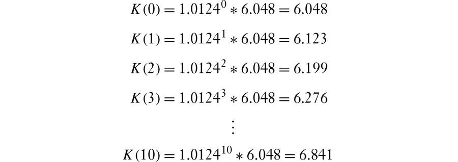
As it turns out, the prediction for K(10) is not far from the population estimate for 2010 in Table 1.1. By 2012, the prediction for K(12) reaches 7.012 billion. Despite hefty uncertainties about true population numbers and despite actual changes in the supposedly constant value of A, our formula gives a fairly realistic picture of overall population growth. It is sobering that a billion people have been added to the human head count in so short a time as a dozen years.

1.2 The Growth Rate R

The Balancing Equation for a closed population led in the last section to an equation for population growth,

Built into this equation is the assumption that the ratio of births to population size B(t)/K(t) and the ratio of deaths to population size D(t)/K(t) are not changing enough to matter over the period from t = 0 to t = T. (We generally use small “t” to stand for time in general, and capital “T” to stand for a particular time like the end of a period.)

When births exceed deaths, A is bigger than 1, and the population is increasing...