Diagram Genus, Generators, and Applications

Alexander Stoimenow

• Publisher: Chapman and Hall/CRC
• Year: 2018
• Print ISBN: 9780367831493
• eBook ISBN: 9781315359984
• Topic: Mathematics
• Subtopic: Arithmetic
• Index: Mathematics

In knot theory, diagrams of a given canonical genus can be described by means of a finite number of patterns ("generators"). Diagram Genus, Generators and Applications presents a self-contained account of the canonical genus: the genus of knot diagrams. The author explores recent research on the combinatorial theory of knots and supplies proofs for a number of theorems.

The book begins with an introduction to the origin of knot tables and the background details, including diagrams, surfaces, and invariants. It then derives a new description of generators using Hirasawa's algorithm and extends this description to push the compilation of knot generators one genus further to complete their classification for genus 4. Subsequent chapters cover applications of the genus 4 classification, including the braid index, polynomial invariants, hyperbolic volume, and Vassiliev invariants. The final chapter presents further research related to generators, which helps readers see applications of generators in a broader context.

Chapter 1

Introduction

1.1 The beginning of knot theory

1.2 Reidemeister moves and invariants

1.3 Combinatorial knot theory

1.4 Genera of knots

1.5 Overview of results

1.5.1 General generator estimates

1.5.2 Compilation of knot generators of genus 4

1.5.3 Unknot diagrams

1.5.4 Non-triviality of the link polynomials

1.5.5 Signature of positive knots

1.5.6 Braid index and Bennequin surfaces

1.5.7 Properties of the Alexander polynomial of alternating knots

1.6 Issues of presentation

1.7 Further applications

1.1 The beginning of knot theory

In the late 19th century, W. Thomson (“Lord Kelvin”), P. G. Tait and J. Maxwell initiated the vortex-atom theory in an attempt to explain the structure of the universe. They believed that a super-substance – ether – makes up all matter and that atoms are knotted tubes of ether. Knotting is thereby understood as tying a piece of rope and then identifying both of its ends so that the tying cannot be any more undone.

Thus, in the realm of constructing a periodic table of elements, Tait began cataloging the simplest knots. He depicted knots (as we still do today) by diagrams, consisting of a (smooth) plane curve with transverse self-intersections, or crossings. At each crossing, one of the two strands passes over the other. The above term “simplest” refers to the number of crossings of the diagram.

We can define the crossing number of a knot as the minimal crossing number of all its diagrams and can say that Tait sought the list of knots with a given (small) crossing number.

There is not much difficulty in creating arbitrarily complicated diagrams of the same knot from a given one; thus, the non-trivial question is whether and to what extent one can reduce the crossing number. This question is very difficult in general, being one of the cornerstones around which all of knot theory was built. However, in certain situations, the answer is easy. In diagrams of the form

the depicted crossing can be easily eliminated (see Figure 2.1). We call such diagrams reducible, and all others reduced.

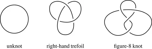
Tait’s list sought to present each knot by exactly one diagram. This requires that knots from different diagrams should be inequivalent in the sense that one cannot turn a (closed) piece of rope which is knotted one way into a piece knotted another way without cutting the rope. The simplest knots are shown in Figure 1.1. The leftmost one, of crossing number 0, is the trivial knot or unknot. It has some special importance, much like the unit element in a group.

FIGURE 1.1: The simplest knots

Tait’s first table went to 7 crossings. His accomplishment entitles him to be called the first knot theorist. However, Tait worked mainly by intuition. He had at his time no rigorous tools to show knots inequivalent. Little, Kirkman, and later Conway [Co] and others took over and continued his work. The efforts to compile knot tables have gone on for more than a century after those early pioneers even though Tait’s vortex-atom theory has long been dismissed. The last manually compiled tables were apparently completed in the 1980’s for 11 crossing knots [Co, Ca, Pe2]. In the modern computer age, tables have reached knots of 17 crossings, with millions of entries. An account on knot tabulation is given—with emphasis on its history—in [S], and from a more contemporary point of view in [HTW, H]. See also §2.3 below.

Right from the start of knot tabulation, a suggestive property attracted some attention. A diagram is called alternating if the curve passes crossings interchangingly over-under like

. A knot is alternating if it has such a diagram. It seems to remain unclear whether Tait was convinced certain properties hold for all knots or just for alternating knots. The knots in Figure 1.1 are alternating. In fact, so are all knots up to 7 crossings, cataloged by Tait, and at least a large portion of the slightly more complicated ones he saw during his lifetime from his successors’ work (even though it is now known that alternation is a rare property for generic crossing numbers [Th3]). Thus, certainly Tait was guided by evidence from alternating diagrams. This evidence would prove misleading in some cases (see the end of Section 2.8.3), but two of his main conjectures stood for a long time.

Conjecture 1.1.1 (Tait’s Crossing Conjecture) A reduced alternating diagram has minimal crossing number (for the knot it represents).

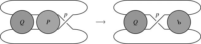
FIGURE 1.2: A flype near the crossing p.

Conjecture 1.1.2 (Tait’s Flyping Conjecture) Alternating diagrams of the same knot are related by a sequence of flypes (shown in Figure 1.2).

1.2 Reidemeister moves and invariants

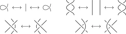
A few decades after Tait, the work of Alexander, Reidemeister and others began to put knot theory onto a mathematical footing. Reidemeister showed that three types of local moves suffice to interrelate all diagrams of the same knot.

These moves are local in the sense that they only alter a fragment of the diagrams, as shown above. The concept of local changes of diagrams (not necessarily preserving the underlying knot or link) is a central theme in knot theory and even more so for this book. Thus, from now on we will understand that whenever a local move is depicted to change between two diagrams, only the altered part will be depicted while the rest of the diagrams will be assumed to be equal.

To distinguish two knots thus translates into the question how to prove that two diagrams (of these knots) are not connected by a sequence of Reidemeister moves. The problem is that such a sequence may be arbitrarily long and pass through very complicated intermediate diagrams. (There is a fundamental issue that one can to some extent control these sequences [HL], and how to do so. We will treat this problem in §5.6.)

Excluding a sequence of Reidemeister moves is done with the help of an invariant, that is, a map

$\left\{\text{knot diagrams}\right\}\text{}\to \text{some domain ,}$

whose value in the domain does not change (is invariant) when the argument (diagram) is changed by a Reidemeister move. Thus, if two diagrams give different invariants, they cannot be related by Reidemeister moves, and hence, they must represent distinct knots. For the value domain of the invariant one thus seeks a set whose objects are easy to distinguish yet which is large enough to allow the invariant to take many different values. The domain will for us usually be the ring of integers, or of (Laurent) polynomials with integer coefficients. Clearly there are many different polynomials, and one can more easily compare coefficients than wondering about a long sequence of Reidemeister moves. Another obvious desirable feature of an invariant is that we can easily evaluate it from a diagram.

Alexander’s contribution was to construct precisely such an invariant. Using his methods, Tait’s knot lists would be proven correct. The Alexander polynomial [Al] remained—and still remains—a main theme in knot theory for decades to come. Let us observe, though, that we actually already came across one other knot invariant (here with values in ℕ), the crossing number. It is an invariant directly by definition, being defined on the whole Reidemeister move equivalence class of diagrams. However, this definition makes it difficult to evaluate from a diagram; moreover, many knots have equal crossing numbers. In contrast, the Alexander’s polynomial can be calculated readily by several procedures (see §2.8.2) and easily distinguishes most knots.

1.3 Combinatorial knot theory

The Alexander polynomial was, from its very beginning, connected to topological features of knots. This topological viewpoint remained a status quo in knot theory research for decades, until in the 1980’s a new chapter was opened by V. Jones with the discovery of a successor to Alexander’s polynomial. The developments the Jones polynomial V [J] has sparked in the 30 years since its appearance are impossible to even vaguely sketch in completeness. Immediately after the Jones polynomial, the skein (HOMFLY-PT), BLMH, Kauffman, and other polynomial invariants appeared, and later Vassiliev [BN3] and quantum invariants. A good related (though still partial, and now no longer very recent) account was given by Birman [Bi].

One of the first achievements of the Jones polynomial, though, was the solution of Tait’s conjectures for alternating knots. The Crossing conjecture was proved by Kauffman [Kf2], Murasugi [Mu, Mu2], and Thistlethwaite [Th4] (see Theorem 2.8.5 below). Kauffman’s proof uses a calculation procedure for V called state model. This state model also gives a very elementary proof that the Jones polynomial is an invariant. (Kauffman had previously developed a similar model for the Alexander polynomial, too [Kf3].) Tait’s Flyping conjecture was resolved a few years later by Menasco and Thistlethwaite [MT] (Theorem 2.6.2 below), mostly by using geometric techniques, though again with some (now subordinate) appearance of the Jones polynomial.

The Jones polynomial and its successors are different from the Alexander polynomial in many ways. One manifestation of this difference is the slow progress toward an important long-standing question of Jones. (We will return to this problem in §5.5.)

Question 1.3.1 Does the Jones (or skein, etc.) polynomial detect the unknot? That is, if a knot has polynomial 1, is it the unknot?

For the Alexander polynomial, our topological understanding has long answered the question (negatively). But attempts to gain topologically more understanding of the newer polynomials failed to a large extent, and thus mathematicians went on looking for other ways. One of these ways was the development of combinatorial knot theory, which is the study of combinatorial properties of knot and link diagrams, a theme to dominate this book. I will focus on a particular piece of this area, developed mainly in my own previous work, with an extensive study of canonical genus. Below I am going to introduce this subject and give an overview of the work in this monograph.

1.4 Genera of knots

Introducing the genus g(K) of a knot K, Seifert [Se] gave a construction of compact oriented surfaces in 3-space bounding the knot (Seifert surface) by an algorithm starting with some diagram of the knot (see [Ad, §4.3] or [Ro]). The surface given by this algorithm is called canonical. A natural problem is when the diagram is genus-minimizing, or of minimal genus, that is, its canonical Seifert surface has minimal genus among all Seifert surfaces of the knot. This problem has been studied over a long period. First, the minimal genus property was shown for alternating diagrams, independently by Crowell [Cw] and Murasugi [Mu2]. Their proof is algebraical, using the Alexander polynomial Δ [Al] and the inequality max deg Δ ≤ g (which thus they proved to be exact for alternating knots). Later Gabai [Ga] developed a geometric method using foliations and showed that this...

Table of contents

• Cover
• Title Page
• Copyright Page
• Table of Contents
• Preface
• List of Figures
• List of Tables
• Symbol Description
• 1 Introduction
• 2 Preliminaries
• 3 The maximal number of generator crossings and ∼-equivalence classes
• 4 Generators of genus 4
• 5 Unknot diagrams, non-trivial polynomials and achiral knots
• 6 The signature
• 7 Braid index of alternating knots
• 8 Minimal string Bennequin surfaces
• 9 The Alexander polynomial of alternating knots
• 10 Outlook
• Bibliography
• Glossary
• Index