Local Polynomial Modelling and Its Applications

Monographs on Statistics and Applied Probability 66

Jianqing Fan

• Publisher: Routledge
• Year: 2018
• ISBN:
  9781351434805
• Edition: 1
• Topic: Mathematics
• Subtopic: Probability & Statistics
• Index: Mathematics

Data-analytic approaches to regression problems, arising from many scientific disciplines are described in this book. The aim of these nonparametric methods is to relax assumptions on the form of a regression function and to let data search for a suitable function that describes the data well. The use of these nonparametric functions with parametric techniques can yield very powerful data analysis tools. Local polynomial modeling and its applications provides an up-to-date picture on state-of-the-art nonparametric regression techniques. The emphasis of the book is on methodologies rather than on theory, with a particular focus on applications of nonparametric techniques to various statistical problems. High-dimensional data-analytic tools are presented, and the book includes a variety of examples. This will be a valuable reference for research and applied statisticians, and will serve as a textbook for graduate students and others interested in nonparametric regression.

CHAPTER 1

Introduction

Regression analysis is one of the most commonly used techniques in statistics. The aim of the analysis is to explore the association between dependent and independent variables, to assess the contribution of the independent variables and to identify their impact on the dependent variable. The main theme of this book is the application of local modelling techniques to various regression problems in different statistical contexts. The approaches are data-analytic in which regression functions are determined by data, instead of being limited to a certain functional form as in parametric analyses. Before we introduce the key ideas of local modelling, it is helpful to have a brief look at parametric regression.

1.1 From linear regression to nonlinear regression

Linear regression is one of the most classical and widely used techniques. For given pairs of data (X_i, Y_i),i = 1,…,n, one tries to fit a line through the data. The part that cannot be explained by the line is often treated as noise. In other words, the data are regarded as realizations from the model:

$Y=\alpha +\beta X+\text{error}\text{.}$

(1.1)

The error is often assumed to be independent identically distributed noise. The main purposes of such a regression analysis are to quantify the contribution of the covariate X to the response Y per unit value of X, to summarize the association between the two variables, to predict the mean response for a given value of X, and to extrapolate the results beyond the range of the observed covariate values.

The linear regression technique is very useful if the mean response is linear:

$E(Y|X=x)\equiv m(x)=\alpha +\beta x.$

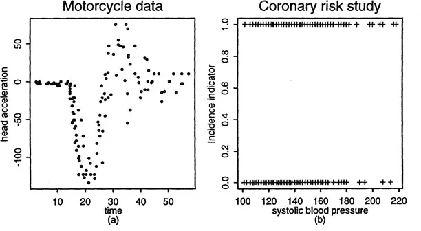
This assumption, however, is not always granted. It needs to be validated at least during the exploration stage of the study. One commonly used exploration technique is the scatter plot, in which we plot X_i against Y_i, and then examine whether the pattern appears linear or not. This relies on a vague ‘smoother’ built into our brains. This smoother cannot however process the data beyond the domain of visualization. To illustrate this point, Figure 1.1 gives two scatter plot diagrams. Figure 1.1 (a) concerns 133 observations of motorcycle data from Schmidt, Mattern and Schüler (1981). The time (in milliseconds) after a simulated impact on motorcycles was recorded, and serves as the covariate X. The response variable Y is the head acceleration (in g) of a test object. It is not hard to imagine the regression curve, but one does have difficulty in picturing its derivative curve. In Figure 1.1 (b), we use data from the coronary risk-factor study surveyed in rural South Africa (see Rousseauw et al. (1983) and Section 7.1). The incidence of Myocardial Infarction is taken as the response variable Y and systolic blood pressure as the covariate X. The underlying conditional probability curve is hard to image. Suffice to say that ‘brain smoothers’ are not enough even for scatter plot smoothing problems. Moreover, they cannot be automated in multidimensional regression problems, where scatter plot smoothing serves as building blocks.

Figure 1.1. Scatter plot diagrams for motorcycle data and coronary risk-factor study data.

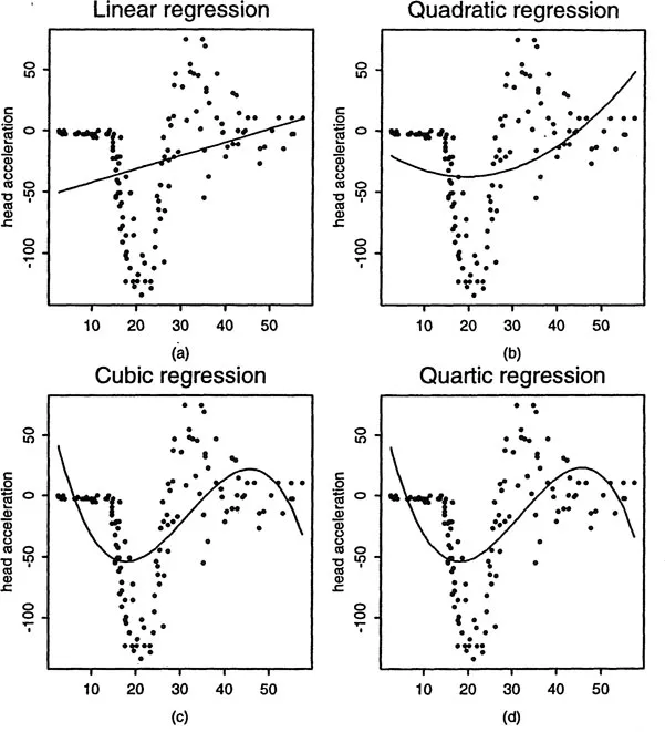
What can we do if the scatter plot appears nonlinear such as in Figure 1.1? Linear regression (1.1) will create a very large modelling bias. A popular approach is to increase the number of parameters by using polynomial regression. Figure 1.2 shows such a family of polynomial fits, which have large biases. While this approach has been widely used, it suffers from a few drawbacks. One is that polynomial functions are not very flexible in modelling many problems encountered in practice since polynomial functions have all orders of derivatives everywhere. Another is that individual observations can have a large influence on remote parts of the curve. A third point is that the polynomial degree cannot be controlled continuously.

Figure 1.2. Polynomial fits to the motorcycle data. The modelling bias is large since the family of polynomial functions is smooth everywhere.

1.2 Local modelling

There are several ways to repair the drawbacks of polynomial fitting. One is to allow possible discontinuities of derivative curves. This leads to the spline approach. The locations of discontinuity points, called knots, can be selected by data via a smoothing spline method or a stepwise deletion method. See Section 2.6. Another possible proposal is to expand the regression function into an orthogonal series, then choose a few useful subsets of the basis functions, and use them to approximate the regression function. Th...