A trivial example
Before formally defining statistical model, I will begin with a trivial example model that demonstrates some of the fundamental ideas about models. Growing up in the United States, I became accustomed to thinking about temperature on the Fahrenheit scale. I know how chilly 40°F is, and I know how warm 75°F is. In Canada, where I now live, temperature is usually reported on the Celsius scale. Unfortunately, I do not automatically have a good sense of what a temperature such as 13°C feels like (should I wear a jacket if I go outside?), so I find that I am constantly converting temperatures reported in Celsius into the approximate Fahrenheit temperature in my head. Of course, there is a known, precise relation between °F and °C, but the conversion isn’t always easy for me to calculate in my head, so I use an approximation that I can calculate quickly. Specifically, I multiply the temperature in °C by two and add 30 to arrive at a value that I know is at least near the temperature in °F.
This approximation is my model for °F given the reported °C, and it can be expressed using the following mathematical equation:
The hat symbol (^) over F on the left-hand side of the equation indicates that the formula produces a
predicted value for °F given a particular value for °C. That is, the value for °C is known, or observed, whereas the value for
is unobserved. (The predicted value is also known as the
model-implied or
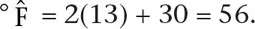
fitted value.) So if I am told that it is 13°C outside and I am wondering whether I should wear a jacket, then I can quickly calculate
Thus, my predicted value for the temperature on the Fahrenheit scale is
= 56, which is not terribly cold but chilly enough that I will probably put on a jacket.
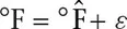
Now, I know that my model does not usually produce the actual, precise value for °F given some temperature in °C. That is, deriving the true °F using this approximation is error-prone, and so another way I can write the model is
where ε is the error term representing the inaccuracy involved in reproducing the true °F using this formula. Next, with some simple algebra, we see that we can substitute Equation 1.1 into Equation 1.2 such that
or
Thus, the error,
ε, gives the difference between the true temperature on the Fahrenheit scale (°F) and the temperature on the Fahrenheit scale predicted by the model (
). Equations 1.1 and 1.2 are different ways of expressing the same model for the relation between °C and °F.
All statistical models are like my temperature model in Equation 1.1 in that they generate predicted values for some outcomes but do so with error. Of course there is an established, true relation between the Fahrenheit and Celsius scales, specifically
Note that Equation 1.4 is not really a model because there is no error term; given a value for °C, we can use Equation 1.4 to calculate the exact, true value for °F.
We can also use Equation 1.4 to evaluate the quality of the model expressed in Equations 1.1 and 1.2. That is, we can use Equation 1.4 to calculate values for the model’s error term,
ε, across different values of °C; in other words, we can use Equation 1.4 to find out how well our predicted values,
, reproduce the true values, °F. For example, if it is 0°C outside (i.e., the temperature at which water freezes), the true °F is 1.8(0) + 32 = 32°F, but the model’s predicted value is 2(0) + 30 = 30°
. Thus, the model is inaccurate by 2°F, or using Equation 1.3, we have
ε = 32 − 30 = 2. So although it’s not precise, the model does a reasonably good job of predicting °F when °C is 0, or freezing. But how well does the model do when, for example, it’s 13°C? Will the model lead to me being too warm in a light jacket, or will I wish that I had put on something heavier? Again, using Equation 1.4, the true °F corresponding to 13°C is 55.4°F, and now
ε = −0.6, which is reasonably accurate given the model’s purpose; that is, I am unlikely to regret my decision to wear a jacket.
To get a more complete picture of how good the model is across a wider range of values for °C, we can plot Equations 1.1 and 1.4 in the same graph, as shown in
Figure 1.1. I have chosen a range of −15°C to 45°C for the
x-axis to represent the wide range of outside temperatures experienced in a given year in North America (having lived in Phoenix, Arizona, and Toronto, I am familiar with both extremes). Clearly, Equations 1.1 and 1.4 are both equations for straight lines but with different intercept and slope values. But in the figure, we see that the lines cross above 10°C, where both the predicted value
and the true value °F equal 50. Thus, for 10°C, the model perfectly reproduces the true °F (i.e.,
ε = 0). To the left of 10°C, the line for the predicted values is below the line for the true values, indicating that when the temperature is below 10°C, the model underestimates the true °F and the corresponding values for the error term
ε are all positive. To the right of 10°C, the predicted line is above the true line, indicating th...