Research Methods for Public Health

Stuart McClean, Issy Bray, Nick de Viggiani, Emma Bird, Paul Pilkington

• Publisher: SAGE Publications Ltd
• Year: 2019
• Print ISBN: 9781526430014, 9781526430007
• eBook ISBN: 9781526485526
• Edition: 1
• Topic: Medicine
• Subtopic: Public Health, Administration & Care

Research Methods for Public Health offers an in-depth introduction to the theories, concepts, approaches and practices, relevant to research methods in a public health setting. Informed by a socio-ecological model of public health, the book uses real world research examples and contemporary social, political and environmental themes of public health that reflect UK and international contexts.

 

The book provides a straightforward approach to developing a research project and applying methods in practical and realistic ways, using an innovative, integrative approach that combines methodologies. The authors have moved away from traditional approaches to research methods, and include chapters on primary quantitative, qualitative and mixed methods research, evidence synthesis approaches, critical appraisal, research governance and ethics, and dissemination.

 

Essential reading for postgraduate students, researchers and public health practitioners, or individuals preparing for the UK Faculty of Public Health Part A examination.

Part 1 Quantitative Methods for Public Health

1 Epidemiology

Chapter Summary

This chapter is divided into two sections. The first introduces the subject of epidemiology in the context of public health, and the key concepts of chance, bias, confounding and causation. The second describes the most common epidemiological study designs, and finishes by considering how these can be applied to the complex interventions and settings often encountered in public health.

Introduction to epidemiology

A classic definition of epidemiology is ‘the study of the distribution and determinants of health-related states or events in specified populations and the application of this study to the control of health problems’ (Last, 2001: 55). This definition stresses that we are interested in the health of populations rather than individuals, and the factors associated with health outcomes. Epidemiology provides the evidence for evidence-based healthcare, by using numbers to estimate and compare risks, either for different subgroups of the population or according to different levels of exposure. More broadly, epidemiology is a quantitative approach to answering questions relating to population health.

Public health research often uses both qualitative and quantitative analysis, and epidemiology is just one of several tools available to public health researchers. For example, an epidemiological approach to determining whether hip protectors are effective in preventing fractures among older people in residential care might select an appropriate study design, such as a randomised controlled trial (RCT) in which half of a sample of nursing homes are provided with hip protectors and half are not. If a large RCT concluded that there was only limited evidence of effectiveness in this population, you might jump to the conclusion that this is not a good use of resources, and rule out this intervention. But you don’t have the full picture – what if the people offered the hip protectors don’t want to wear them, and are therefore not complying with the intervention being tested? Then some qualitative work is needed to understand the experience of older people wearing hip protectors, and barriers to their use. This could inform further research into alternative designs with potentially higher rates of compliance. Assuming different designs come at different costs, then a comparison of the relative cost-effectiveness of each would be useful. Other tools, such as qualitative research and health economics, are therefore required to complement epidemiology (Bowling, 2014).

Framing a question

Before we can consider the most appropriate epidemiological study design in a particular situation, we have to be clear about our research question. A useful framework for doing this is PICO. In public health, P stands for ‘population’ (rather than ‘patient’ as in traditional evidence-based medicine). This highlights the key difference between public health and clinical professions – we are considering whole populations rather than individual patients. I stands for ‘intervention’ (or ‘exposure’ in non-experimental studies). C stands for ‘comparison’ (having a control or comparison group is a key characteristic of epidemiological studies), and O stands for ‘outcome’. So, in any epidemiological study we are considering the effect of an exposure or intervention on a particular health outcome, but we also need to define what this is being compared to and in which particular population.

Box 1.1 PICO: Population, Intervention, Comparison, Outcome

Using the hip protector example given above:

• P Older people (e.g. 65+ years) living in residential homes in the UK
• I Provision of hip protectors
• C No provision of hip protectors
• O Fractures

In this example, we have compared the provision of hip protectors to no provision, but it could be that we want to compare the provision of a new type of hip protector with the current market leader. Then the comparison would be with another intervention, rather than no intervention.

In epidemiology, the intervention or exposure is sometimes referred to as the independent variable, explanatory variable or risk factor, while the health or social outcome that we are interested in may be described as the dependent variable. So, an epidemiological study uses quantitative techniques to assess the effect of a particular exposure or intervention on a health outcome of interest in a defined population by comparing groups with different levels of exposure. Before going on to describe the main epidemiological study designs in further detail, we will consider some common problems in epidemiology which researchers must be aware of. These topics of chance, bias and confounding are dealt with in greater depth in epidemiology textbooks such as Gordis (2013) and Rothman (2012).

Chance

Epidemiological studies are usually based on samples drawn from the population of interest, because it is not normally possible to measure exposures and outcomes on the entire population. For example, if I want to assess whether open-water swimming is a risk factor for a particular waterborne illness in the southwest of England, I am unlikely to be able to gather information on frequency of open-water swimming for every individual in this population, but I can survey a sample. The next chapter will focus on different methods of sampling. If, in my sample, I find that there is evidence of an association, in other words that open-water swimming does appear to increase the risk of the illness, then how confident should I be that this association is real? Is it possible that if I took a different sample then I might get a different result? Most people intuitively trust results based on a large sample more than those derived from a small sample. So, if I told you that I had surveyed 10 people on this issue and found an association, you might be dubious. If I told you I had surveyed 1,000 people and found an association between open-water swimming and waterborne illness, you would probably be more inclined to believe me. This is correct; larger samples are more reliable. Statistics can be used to quantify how confident we should be in the study’s results. Confidence intervals can be calculated for our results, which take into account the size of the sample, and other characteristics of the study design and sample. ‘p-values’ are sometimes also calculated to quantify the probability that the difference we observed is due to chance (how likely is it that we would have got the observed difference, or a larger difference, if there was actually no association between open-water swimming and waterborne illness?). Since p stands for ‘probability’, it is on a scale of 0 to 1, and it is important to interpret the p-value as a value on a continuum, to describe the strength of the evidence, rather than using an arbitrary cut-off for the p-value to determine whether a result is ‘statistically significant’ or not. Traditionally, this arbitrary cut-off has been set at 0.05 (or 5%), and used to interpret a p-value of less than 0.05 as ‘significant’ (in other words there is evidence of an association or a difference) and a value greater than 0.05 as non-significant (no evidence of an association/difference). When presenting your own research, it is good practice to present confidence intervals (Gardner and Altman, 1986), and if p-values are also used then the actual p-value should be given (rather a statement about the statistical significance or otherwise of the results). When reading or critiquing published research, remember to take into account the width of the confidence intervals rather than focusing on the overall estimate, because they will often indicate a very wide range of likely values, in other words a lack of confidence about what is actually going on in the population.

Bias

Bias refers to a systematic error in the way a study is conducted, analysed or reported, which means that the results cannot be trusted. There are many different types of bias, as illustrated by the following examples. In the case of the study looking at open-water swimming and waterborne illness, the study could be biased if it were conducted at a particular time of year when the waterborne pathogen of interest was particularly prevalent – this might over-estimate, and therefore exaggerate, the risks more usually associated with open-water swimming. This is a form of sampling bias, in that the sample was not taken at a representative time. Imagine next that I am surveying patients about their satisfaction with a smoking cessation service. It seems sensible to wait until patients have completed all planned sessions before asking them to evaluate the service. But if half the patients drop out before completing all sessions, and so do not get surveyed, it is reasonable to assume that my results will be positively skewed by not including those who did not complete, and quite likely were less satisfied with the service, in other words the results are biased by attrition. In the case of a trial of hip protectors in residential settings for older people, the researchers might find a reduction in risk for pelvic fractures but no evidence of a reduction in risk for hip fractures associated with the intervention. If only the results for pelvic fractures are presented, then this will give an overly optimistic view of the effectiveness of the intervention, and this is known as reporting bias. Taking this example a step further, if it were the case that ten such trials have been conducted in the last five years, and imagine that half have found evidence of a protective effect of providing hip protectors and half have not. If the five ‘negative’ finding studies are not published in peer-reviewed journals (either because the authors do not think it is worth writing up, or because this is not a sufficiently interesting finding to find its way into a journal), but the five ‘positive’ finding results are accessible in journals, then any review of the subject will conclude that the evidence for providing hip protectors in residential settings for older people is much stronger than it really is. This is due to publication bias, the extent and implications of which are further discussed by Dwan et al. (2013). There are many other forms of bias beyond those mentioned here. The key thing is for researchers to be alert to possible sources of bias in their own research, and in published studies (see, for example, Lundh et al., 2017).

Confounding

Confounding is actually a form of bias, but is so important in epidemiology that it is usually considered as a separate problem. It refers to the very common situation in which the association of interest between an exposure and an outcome is biased by some other factor. This other factor, known as a confounder (or confounding factor), is associated with both the exposure and the outcome.

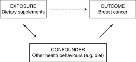
Consider a study looking at the association between dietary vitamin supplementation and breast cancer, to test the hypothesis that dietary supplementation reduces the risk (see Figure 1.1a). If a negative association is found (i.e. supplementation is associated with lower rates of cancer), then this could be taken in support of the hypothesis. This apparent association is denoted by the dotted arrow in Figure 1.1a. However, it is quite likely that those people in the sample who take vitamin supplements are more health conscious than those who don’t, and therefore engage in other health behaviours likely to reduce their risk of cancer (in terms of diet, and alcohol and tobacco use). This association is denoted by the double-headed solid arrow in Figure 1.1a.

Figure 1.1a Example of confounding by health behaviours

It may be these other health behaviours that reduce the risk of breast cancer (denoted by another solid arrow), rather than the dietary supplementation. Another example is the apparent association between breastfeeding and the subsequent body mass index (BMI) of the child (see Figure 1.1b). Breastfeeding in the UK is socially patterned (solid double-headed arrow). Since higher socio-economic status is associated with a range of dietary and lifestyle factors which are likely to lead to lower BMI (also denoted by a solid arrow), it appears that breastfeeding is associated with lower BMI in children (dotted arrow). Interestingly, this social patterning does not exist in every country, and data from Brazil has been used to demonstrate that in the absence of an association between breastfeeding (the exposure) and socio-economic status (the confounder), there is no evidence of an association between breastfeeding and child BMI (Brion et al., 2011).

Figure 1.1b Example of confounding by socio-economic status

Common confounders in epidemiology are age, gender, socio-economic status and ethnicity. While Figure 1.1 shows one confounder operating at a time, in reality there could be several confounders operating at once, including other more specific confounders for the particular association under study. When considering possible confounders, always ask whether it is (or could plausibly be) associated with both the exposure and the outcome. If not, then it is not a potential confounder.

Epidemiology has various methods to deal with confounding at both the study design stage and the analysis stage (and both will be discussed later), but these generally require us to identify and measure these variables for our study population. If we are unaware of certain confounders then we cannot measure them, and this is a problem (though one which is largely overcome by RCTs, as we shall see later). Another problem with most epidemiological study designs is that even though they allow confounders to be measured and taken into account, there is often a degree of ‘residual confounding’. This is because when we try to measure confounders, we often end up with a poor proxy, so our adjustment for confounding is only partial. While age and gender are fairly straightforward to measure,...

Table of contents

• Cover
• Half Title
• Publisher Note
• Title Page
• Copyright Page
• Contents
• List of tables
• List of figures
• About the Authors
• Acknowledgements
• Publisher’s Acknowledgements
• Introduction
• Part 1 Quantitative Methods for Public Health
• 1 Epidemiology
• 2 Sampling
• 3 Collecting Quantitative Data
• 4 Quantitative Data Analysis
• 5 Quality and Rigour in Quantitative Research
• Part 2 Qualitative Methods for Public Health
• 6 Methodological Approaches and Basic Principles
• 7 Accessing and Selecting Cases in Qualitative Research
• 8 Collecting Qualitative Data
• 9 Qualitative Data Analysis
• 10 Quality and Rigour in Qualitative Research
• Part 3 Mixing it Up: Combining Methods and Evidence Synthesis in Public Health
• 11 Mixed Methods Research and Evaluation Design
• 12 Evidence Synthesis Approaches: Systematic Reviews
• 13 Evidence Synthesis Approaches: Meta-ethnography and Realist Synthesis
• Part 4 Applying Research to Public Health Practice
• 14 The Ethics of Public Health Research
• 15 Writing up, Dissemination and Publication
• References
• Index