Biochar

A Guide to Analytical Methods

Balwant Singh, Marta Camps-Arbestain, Johannes Lehmann, Balwant Singh, Marta Camps-Arbestain, Johannes Lehmann

• Publisher: CSIRO PUBLISHING
• Year: 2017
• Print ISBN: 9781486305094
• eBook ISBN: 9781486305117
• Topic: Physical Sciences
• Subtopic: Chemistry
• Index: Chemistry

Interest in biochar among soil and environment researchers has increased dramatically over the past decade. Biochar initially attracted attention for its potential to improve soil fertility and to uncouple the carbon cycle, by storing carbon from the atmosphere in a form that can remain stable for hundreds to thousands of years. Later it was found that biochar had applications in environmental and water science, mining, microbial ecology and other fields.

Beneficial effects of biochar and its environmental applications cannot be fully realised unless the chemical, physical, structural and surface properties of biochar are known. Currently many of the analytical procedures used for biochar analysis are not well defined, which makes it difficult to choose the right biochar for an intended use and to compare the existing data for biochars. Also, in some instances the use of inappropriate procedures has led to erroneous or inaccurate values for biochars in the scientific literature.

Biochar: A Guide to Analytical Methods fills this gap and provides procedures and guidelines for routine and advanced characterisation of biochars. Written by experts, each chapter provides background to a technique or procedure, a stepwise guide to analyses, and includes data for biochars made from a range of feedstocks common to all presented methods. Discussion about the unique features, advantages and disadvantages of a particular technique is an explicit focus of this handbook for biochar analyses.

Biochar is primarily intended for researchers, postgraduate students and practitioners who require knowledge of biochar properties. It will also serve as an important resource for researchers, industry and regulatory agencies dealing with biochar.

1 Sampling, storage and preparation of biochar for laboratory analysis

Isabel Hilber, Hans-Peter Schmidt and Thomas D. Bucheli

INTRODUCTION

Out of the various elements of experimental design, sampling is probably the most underrated one. In light of the fact that sampling errors are typically one to two, even up to three orders of magnitude greater than analytical ones (Gy 2004a; Petersen et al. 2005), this can have significant consequences for data precision and reliability of results.

In this chapter, we will show that biochar is a constitutional and distributional heterogeneous material. As such, its sampling is prone to be non-probabilistic and thus unrepresentative, leading to incorrect sampling errors. Generally, this holds for pure biochars, as well as for biochar diluted with other matrices, such as soil, compost or manure.

While representative sampling and sample preparation of biochar with correct mass reduction (in the field as well as in the laboratory) is far from trivial, the theory of sampling introduced by Pierre Gy some 50 years ago (Gy 2004a; Petersen et al. 2005) provides a theoretical and practical framework to which the biochar community can, and should, resort more systematically.

As biochar is a highly sorptive material, it is prone to adsorb air, water and other compounds after sampling. Such adsorbed compounds may then react with biochar surfaces and minerals (Amonette and Joseph 2009). Hence, alteration or contamination during transport, storage and sample preparation for analysis can contribute to further biases.

Without being exhaustive, this chapter provides a qualitative guidance for adequate biochar sampling, storage and preparation for laboratory analysis. Key references are listed and the reader is referred to them for further details.

THE HETEROGENEITY OF BIOCHAR

According to Gy (2004a), as with any particulate discrete material, biochar is a constitutional and distributional heterogeneous matter. We will explain and illustrate these heterogeneities in the next two sections on the basis of two datasets.

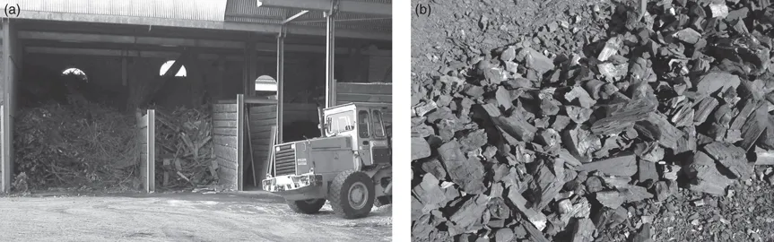
Figure 1.1: Examples of constitutional and distributional heterogeneous material. (a) Lop and wood residues. (b) A possible biochar.

Heterogeneity on laboratory scale

The feedstock of biochar is diverse (Fig. 1.1a) and so is the product after pyrolysis (Fig. 1.1b). Biochar exhibits constitutional heterogeneity,¹ which means that the fragments or particles do not have a strictly identical chemical and/or physical composition. Constitutional heterogeneity can be reduced, e.g. by crushing, grinding and milling. To illustrate constitutional heterogeneity, we performed a small experiment. We sieved several kilograms of three different biochars and measured their polycyclic aromatic hydrocarbon (PAH) concentrations in the different particles (Fig. 1.2, left y-axis, columns). All biochars had the highest PAH contents in the two smallest particle size categories (d (diameter) <0.05 mm and 0.05 mm ≤ d <0.25 mm). The mass of the two smallest particle size fractions consisted of maximally 20% of the total mass (Fig. 1.2, right y-axis, dots) irrespective of the biochar feedstock. Thus, the constitution of the biochar was physically and chemically heterogeneous. This also holds true for elements like C, H, O and any other investigated analytes of the biochar. Constitutional heterogeneity of PAHs is primarily due to their recondensation from the gas phase on the surface of the biochar during the pyrolysis. This process is controlled by surface area and not mass of the sorbent (Bucheli et al. 2015).

The distributional heterogeneity of biochar largely results from its constitutional heterogeneity. The groups or neighbouring constituents do not have a strictly identical composition or are not evenly distributed in the lot. Distributional heterogeneity can be reduced by mixing or blending. Every material exhibits constitutional and distributional heterogeneity, which must be accounted for during sampling.

Heterogeneity on field scale: a case study

A sample can be taken in different ways (Thompson 2001; Gy 2004a), depending on the rationale behind the sampling. Simple grab-sampling is the procedure performed most often, but is almost always non-correct and therefore a ‘no-go’. While the specimen is the result of a non-correct sampling procedure, the sample represents the correct way. In a field-scale case study with a biochar lot of 750 kg, Bucheli et al. (2014) compared PAH and element concentration means and relative standard deviation (RSD, standard deviation over mean concentration) of a specimen (n = 5) with a sample (n = 4). The RSD is a measure for precision in the field of analytical chemistry. The hypothesis underlying this case study was that the precision of the specimen was smaller (high RSD) than that of the sample (low RSD).

The pitfall of grab-sampling is that the specimen is easily taken by simply grabbing a small shovel a few times into the biochar lot, which was deliberately done in the case study. This action is a non-correct way because some particles/pieces, particularly in the lower and middle part of the lot, had low to zero probability (not equal probability) of being picked, whereas the ones on the surface had a higher one. Grab-sampling leads to unreliable results due to the unreliable specimen.

Figure 1.2: Illustration of the constitutional (physical and chemical) heterogeneity of biochar. Sum (∑) of the 16 US EPA PAHs (left y-axis) in different particle sizes (d = diameter) of biochars from three different feedstocks and their respective weight as fraction of the total mass (right y-axis).

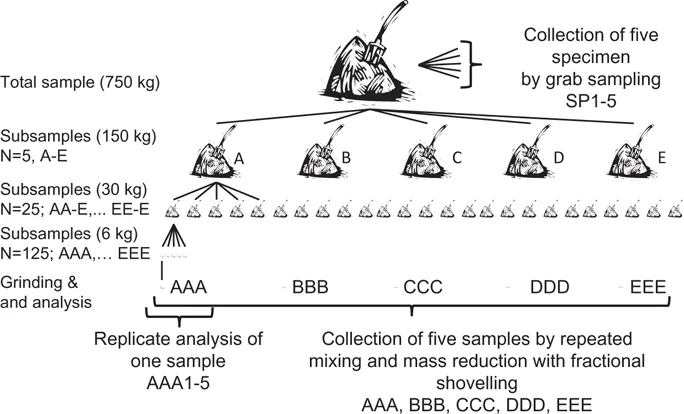
To obtain equal probability for all particles/pieces in a solid material, the lot needs to be mixed and split repeatedly to reduce the distributional heterogeneity. Bucheli et al. (2014) mixed the biochar thoroughly, and systematically split it into five equal heaps. This procedure was repeated three times (Fig. 1.3).

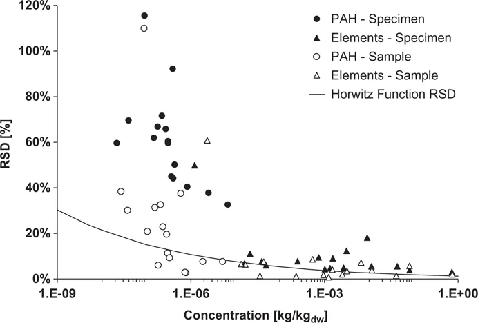
The specimen and samples obtained after grabbing or mixing and splitting were taken to the laboratory and analysed for PAHs and elements. As hypothesised, the samples showed lower RSD than the specimens of both, for PAHs and elements. The average RSD of the specimens and samples were 10% and 7% for all elements and 61% and 24% for all 16 individual PAH compounds, respectively (Fig. 1.4). There are several reasons for the smaller RSD of the elements than the PAHs. First, it is a consequence of the concentration. Horwitz (1982) showed that the coefficient of variation, which is the same as RSD, depends on the concentration of the analyte (Fig. 1.4, black line). The lower the concentration the higher the RSD, and therefore the elements with concentrations in the per mil to mg/kg concentrations showed lower RSD than the PAHs, being in the μg/kg range.

Second, lower RSD of the elements compared to PAHs might be due to the origin of the compounds. The elements were inherent in the feedstock, survived the pyrolysis and might have had a lower distributional heterogeneity than the PAHs. In contrast, PAHs are mostly formed during pyrolysis and are mainly clustered in small particles (Fig. 1.2).

Third, the still too high RSD of the PAH sample in comparison to the Horwitz function is also a consequence of the difficult analysis of PAH in biochar. Typically, PAHs in biochars are dominated by naphthalene but also by fluoranthene and phenanthrene (Bucheli et al. 2015). Naphthalene is a volatile compound and can cross-contaminate other samples that originally had lower concentrations, for instance during parallel extraction solvent evaporation (Hilber et al. 2012), and thereby cause high RSD of replicate analyses.

Figure 1.3: Sampling experiment where a lot of 750 kg biochar was sampled in different ways to obtain specimens and samples. Source: Bucheli et al. (2014) with permission from the publisher.

Consequences of improper sampling

The PAH concentrations (and some of the elements) of the specimen were not trustworthy mostly due to the non-representative sampling. The mean concentration in the specimens for the sum (Σ) of the 16 PAHs was 13.5 ± 5.0 mg/kg_{dry weight (dw)} and for the samples 11.0 ± 0.5 mg/kg_dw. The 90% confidence interval of the Student t-distribution of these concentrations extended the concentrations of 2.9–24.1 mg/kg_dw and of 10.1–12.0 mg/kg_dw for specimens and samples, respectively (Fig. 1.5).

Figure 1.4: Relative standard deviation (RSD) of specimen and sample concentrations of elements and PAHs in the biochar. The black line represents the empirical concentration dependence of RSD for presumably representative samples (Horwitz 1982). Source: Graph modified from Bucheli et al. (2014) with permission from the publisher.

This confidence interval gives a 90% probability that the PAH concentration of every specimen additionally analysed will be in this wide range of 2.9–24.1 mg/kg_dw, which certainly is not very trustworthy. The European Biochar Certificate (EBC 2012) qualifies a biochar with a Σ16 PAH of <4 mg/kg_dw as the premium grade and of <12 mg/kg_dw as the basic grade; above the concentration of 12 mg/kg_dw biochar shall not be sold. In contrast, the sample with its narrow confidence interval (10.1–12.0 mg/kg_dw) indicates a 90% probability that the biochar can be sold under the basic grade according to the EBC (Σ16 PAH <12 mg/kg_dw) as well as under the International Biochar Initiative (IBI 2015).

Figure 1.5: Student t-distribution of the sum (Σ) of the 16 PAHs in (a) the specimens and (b) the samples.

SAMPLING IN PRACTICE

Although the focus of this book is biochar, the theory of sampling and related sampling strategies are also valid for soil–biochar blends. Biochar is often amended to soils for agricultural (Lehmann and Joseph 2009) or remediation purposes (Beesley et al. 2011) and it is important to know its influence on this environmental compartment. A lot of research questions are addressed via pot experiments where soil was treated with biochar (e.g. De la Rosa et al. 2015). None of these materials, in fact no material, will ever be homogeneous (Gy 2004a), neither in a constitutional nor in a distributional way. In practice, we th...

Table of contents

• Cover
• Title
• Copyright
• Contents
• Preface and acknowledgements
• List of contributors
• 1 Sampling, storage and preparation of biochar for laboratory analysis
• 2 Proximate analyses for characterising biochars
• 3 Biochar pH, electrical conductivity and liming potential
• 4 Analysis of biochars for C, H, N, O and S by elemental analyser
• 5 Inorganic carbon
• 6 Dissolved carbon and LC-OCD of biochar
• 7 Determination of cation exchange capacity in biochar
• 8 Determining acidic groups at biochar surfaces via the Boehm titration
• 9 Total elemental analysis of metals and nutrients in biochars
• 10 Available nutrients in biochar
• 11 Polycyclic aromatic hydrocarbons in biochar
• 12 Analysis of biochar porosity by pycnometry
• 13 Guiding principles for measuring sorption of organic compounds on biochars
• 14 Analysis of biochars by 13C nuclear magnetic resonance spectroscopy
• 15 Analysis of biochars using benzene polycarboxylic acids
• 16 Pyrolysis-GC-MS of biochar
• 17 Analysis of biochars by hydropyrolysis
• 18 Biochar analysis by Fourier-transform infra-red spectroscopy
• 19 Carbon near-edge absorption fine structure as a tool for understanding chemical differences in biochars
• 20 X-ray photoelectron spectroscopy analysis of biochar
• 21 X-ray diffraction analysis of biochar
• 22 Stable isotope analysis of biochars
• 23 Application of scanning electron microscopy to the analysis of biochar-related materials
• 24 Thermal analysis for biochar characterisation
• Appendix 1. Biochar samples and their preparation for laboratory analysis
• Appendix 2. Specific surface area and porosity measurements
• Index