Categorical Data Analysis With Sas and Spss Applications

Bayo Lawal, H. Bayo Lawal

• Publisher: Psychology Press
• Year: 2003
• Print ISBN: 9781138003873, 9780805846058
• eBook ISBN: 9781135623296
• Edition: 1
• Topic: Psychology
• Subtopic: History & Theory in Psychology
• Index: Psychology

This book covers the fundamental aspects of categorical data analysis with an emphasis on how to implement the models used in the book using SAS and SPSS. This is accomplished through the frequent use of examples, with relevant codes and instructions, that are closely related to the problems in the text. Concepts are explained in detail so that students can reproduce similar results on their own. Beginning with chapter two, exercises at the end of each chapter further strengthen students' understanding of the concepts by requiring them to apply some of the ideas expressed in the text in a more advanced capacity. Most of these exercises require intensive use of PC-based statistical software. Numerous tables with results of analyses, including interpretations of the results, further strengthen students' understanding of the material. Categorical Data Analysis With SAS(R) and SPSS Applications features:
*detailed programs and outputs of all examples illustrated in the book using SAS(R) 8.02 and SPSS on the book's CD; *detailed coverage of topics often ignored in other books, such as one-way classification (ch. 3), the analysis of doubly classified data (ch. 11), and generalized estimating equations (ch. 12); and *coverage of SAS(R) PROC FREQ, GENMOD, LOGISTIC, PROBIT, and CATMOD, as well as SPSS PROC CROSSTABS, GENLOG, LOGLINEAR, PROBIT, LOGISTIC, NUMREG, and PLUM. This book is ideal for upper-level undergraduate or graduate-level courses on categorical data analysis taught in departments of biostatistics, statistics, epidemiology, psychology, sociology, political science, and education. A prerequisite of one year of calculus and statistics is recommended. The book has been class tested by graduate students in the department of biometry and epidemiology at the Medical University of South Carolina.

Chapter 1

Introduction

In this text, we will be dealing with categorical data, which consist of counts rather than measurements. A variable is often defined as the characteristic of objects or subjects that varies from one object or subject to another. Gender, for instance, is a variable as it varies from one person to another. In this chapter, because variables consist of different types, we describe the variable classification that has been adopted over the years in the following section.

1.1 Variable Classification

Stevens (1946) developed the measurement scale hierachy into four categories, namely, nominal, ordinal, interval and ratio scales. Stevens (1951) further prescribed statistical analyses that are appropriate and/or inappropriate for data that are classified according to one of the four scales above. The nominal scale is the lowest while the ratio scale variables are the highest.

However, this scale typology has seen a lot of critisisms from, namely, Lord (1953), Guttman (1968), Tukey (1961,) and Velleman and Wilkinson (1993). Most of the critisisms tend to focus on the prescription of scale types to justify statistical methods. Consequently, Velleman and Wilkinson (1993) give examples of situations where Steven’s categorization failed and where statistical procedures can often not be classified by Steveen’s measurement theory.

Alternative scale taxonomies have therefore been suggested. One of such was presented in Mosteller and Tukey (1977, chap. 5). The hierachy under their classification consists of grades, ranks, counted fractions, counts, amounts, and balances.

A categorical variable is one for which the measurement scale consists of a set of categories that is non-numerical. There are two kinds of categorical variables: nominal and ordinal variables. The first kind, nominal variables, have a set of unordered mutually exclusive categories, which according to Velleman and Wilkinson (1993) “may not even require the assignment of numerical values, but only of unique identifiers (numerals, letters, color)”. This kind classifies individuals or objects into variables such as gender (male or female), marital status (married, single, widowed, divorced), and party affiliation (Republican, Democrat, Independent). Other variables of this kind are race, religious affiliation, etc. The number of occurrences in each category is referred to as the frequency count for that category. Nominal variables are invariant under any transformations that preserves the relationship between subjects (objects or individuals) and their identifiers provided we do not combine categories under such transformations. For nominal variables, the statistical analysis remains invariant under permutation of categories of the variables.

As an example, consider the data in Table 1.1 relating to the distribution 120 students in an undergraduate biostatistics class in the fall of 2001. The students were classified by their gender (males or females). Table 1.1 displays the classification of the students by gender.

Table 1.1: Classification of 120 students in class by gender

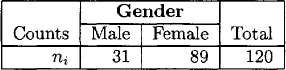
When nominal variables such as variable gender have only two categories, we say that such variables are dichotomous or binary. This kind of variables have been sometimes referred to as the categorical-dichotomous. A nominal variable such as color of hair with categories {black, red, blonde, brown, gray}, which has multiple categories but again without ordering, is referred to (Clogg, 1995) as categoricalnominal.

The second kind of variables, ordinal variables, are where the categories are ordered. Using the definition in Velleman and Wilkinson (1993), if S is an ordinal scale that assigns real numbers in ℜ to the elements of a set P, of observed observations, then

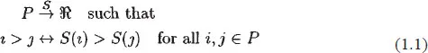
Such a scale S preserves the one-to-one relation between numerical order values under some transformation. The set of transformations that preserves the ordinality of the mapping in (1.1) has been described by Stevens (1946) as being permissible. That is, the monotonic transformation f is permissible if and only if;

Thus for this scale of measurements, permissible transformations are logs or square roots (nonnegative), linear, addition or multiplication by a positive constant.

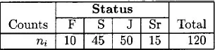
Under an ordinal scale, therefore, the subjects or objects are ranked in terms of degree to which they posses a characteristic of interest. Examples are: rank in graduating class (90th percentile, 80th percentile, 60th percentile); social status (upper, middle, lower); type of degree (BS, MS, PhD); etc. The Likert variable such as the attitudinal response variable with four levels (strongly dissapprove, dissapprove, approve, strongly approve) can sometimes be considered as a partially ordinal variable (a variable with most levels ordered with one or more unordered levels) by the inclusion of the response level “don’t know” or “no answer” category. Ordinal variables generally indicate that some subjects are better than others but then, we can not say by how much better, because the intervals between categories are not equal. Consider again the 120 students in our biostatistics class now classified by their status at the college (freshman, sophomore, junior, or senior). Thus the status variable has four categories in this case.

The results indicate that more than 75% of the students are either sophomores or juniors. Table 1.2 will be referred to as a one-way classification table because it was formed from the classification of a single variable, in this case, status. For the data in Table 1.2, there is an intrinsic ordering of the categories of the variable “status”, with the senior category being the highest level in this case. Thus this variable can be considered ordinal.

Table 1.2: Distribution of 120 students in class by status

On the other hand, a metric variable has all the characteristics of nominal and ordinal variables, but in addition, it is based on equal intervals. Height, weight, scores on a test, age, and temperatures are examples of interval variables. With metric variables, we not only can say that one observation is greater than another but by how much. A fuller classification of variable types is provided by Stevens (1968).

Within this grouping, that is, nominal, ordinal, and metric, the metric or interval variables are highest, followed by ordinal variables. The nominal variables are lowest. Statistical methods applied to nominal variables will also be applicable to either ordinal or interval variables but not vice versa. Similarly, statistical methods applicable to ordinal variables can also be applied to interval variables, again but not vice versa, nor can it be applied to nominal variables since these are lower in order on the measurement scale.

When subjects or objects are classified simultaneously by two or more attributes, the result of such a cross-classification can be conveniently arranged as a table of counts known as a contingency table. The pattern of association between the classificatory variables may be measured by computing certain measures of association or by fitting of log-linear model, logit, association, or other models.

1.2 Categorical Data Examples

Suppose the students in this class have been cross-classified by two variables, gender and status, then the resulting table will be described as a two-way table or a two-way contingency table below (see Table 1.3). Table 1.3 displays the cross-classification of students by gender and status.

Table 1.3: Joint classification of students by status and gender

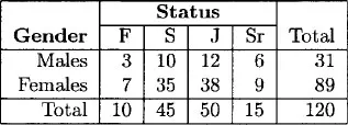
The frequencies in Table 1.3 above indicate that there are 31 male students in this class and 89 female students. Further, the table also reveals that of the 120 students in the class, 38 are females whose status category is junior.

In general, our data will consist of counts {n_i, i=1, 2, …, k} in the k cells (or categories) of a contingency table. For instance, these might be observations for the k levels of a single categorical variable, or for k=IJ cells of a two-way I×J contingency table. In Tables 1.1 and 1.2, k equals 2 and 4 respectively, while k=8 in Table 1.3. We shall treat counts as random variables. Each observed count, ni has a distribution that is concentrated on the non-negative integers, with expected values denoted by m_i=E(n_i). The {m_i} are called expected frequencies, while the {n_i} are referred to as the observed frequencies. Observed frequencies refer to how many objects or subjects are observed in each category of the variable(s).

1.3 Analyses

For the data in Tables 1.1 and 1.2, interest for this type of data usually centers on whether the observed frequencies follow a specified distribution usually leading to what is often referred to as ‘goodness-of-fit test’. For the data in Table 1.3, on the other hand, our interest in this case is often concerned with independence, that is, whether the students’ status is independent of gender. This is referred to as the test of independence. An alternative form of this test is the test of “homogeneity”, which postulates, for instance, that the proportion of females (or males) is the same in each of the four categories of “status”. We will see that both the independence and homogeneity tests lead asymptotically to the same result in chapter 5. We may on the other hand wish to exploit the ordinal nature of the status variable (since there is an hierachy with regards to the categories of this variable). We shall consider this and other situations in chapters 6 and 9, which deals with log-linear model and association analyses of such tables. The various measure of association exhibited by such tables are discussed in chapter 5.

1.3.1 Examp...

Table of contents

• Cover
• Half Title
• Title Page
• Copyright
• Contents
• Preface
• 1. Introduction
• 2. Probability Models
• 3. One-Way Classification
• 4. Models for 2×2 Contingency Tables
• 5. The General I×J Contingency Table
• 6. Log-Linear Models for Contingency Tables
• 7. Strategies for Log-Linear Model Selection
• 8. Models for Binary Responses
• 9. Logit and Multinomial Response Models
• 10. Models in Ordinal Contingency Tables
• 11. Analysis of Doubly Classified Data
• 12. Analysis of Repeated Measures Data
• Appendices
• Table of the Chi-Squared Distribution
• Bibliography
• Subject Index