Juan A. Martinez-Velasco
1.1 Introduction
Power system transient analysis is usually performed using computer simulation tools like the Electromagnetic Transients Program (EMTP), although modeling using Transient Network Analyzers (TNAs) is still done, but decreasingly. There is also a family of tools based on computerized real-time simulations, which are normally used for testing real control system components or devices such as relays. Although there are several common links, this chapter targets only off-line nonreal-time simulations.
Engineers and researchers who perform transient simulations typically spend only a small amount of their total project time running the simulations. The bulk of their time is spent obtaining parameters for component models, testing the component models to confirm proper behaviors, constructing the overall system model, and benchmarking the overall system model to verify overall behavior. Only after the component models and the overall system representation have been verified, one can confidently proceed to run meaningful simulations. This is an iterative process. If there are some transient event records to compare against, more model benchmarking and adjustment may be required.
This book deals with parameter determination and is aimed at reviewing the procedures to be performed for deriving the mathematical representation data of the most important power components in electromagnetic transient simulations. This chapter presents a summary on the current status and practice in this field and emphasizes needed improvements for increasing the accuracy of modeling tasks in detailed transient analysis.
FIGURE 1.1
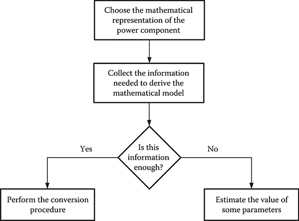
Procedure to obtain a complete representation of a power component. (From Martinez, J.A. et al., IEEE Power Energy Mag., 3, 16, 2005. With permission.)
Figure 1.1 shows a flow chart of the procedure suggested to obtain the complete representation of a power component [1]:
First, choose the mathematical model.
Second, collect the information that could be useful to determine the values of parameters to be specified.
Third, decide whether the available data are enough or not to derive all parameters.
The procedure depicted in Figure 1.1 assumes that the values of the parameters to be specified in some mathematical descriptions are not necessarily readily available and they must be deduced from other information using, in general, a data conversion procedure.
1.2 Modeling Guidelines
An accurate representation of a power component is essential for reliable transient analysis. The simulation of transient phenomena may require a representation of network components valid for a frequency range that varies from DC to several MHz. Although the ultimate objective in research is to provide wideband models, an acceptable representation of each component throughout this frequency range is very difficult, and for most components is not practically possible. In some cases, even if the wideband version is available, it may exhibit computational inefficiency or require very complex data.
Modeling of power components that take into account the frequency-dependence of parameters can be currently achieved through mathematical models which are accurate enough for a specific range of frequencies. Each range of frequencies usually corresponds to some particular transient phenomena. One of the most accepted classifications is that proposed by the International Electrotechnical Commission (IEC) and CIGRE, in which frequency ranges are classified into four groups [2,3]: low-frequency oscillations, from 0.1 Hz to 3 kHz; slow-front surges, from 50/60 Hz to 20 kHz; fast-front surges, from 10 kHz to 3 MHz; and very fast-front surges, from 100 kHz to 50 MHz. One can note that there is overlap between frequency ranges.
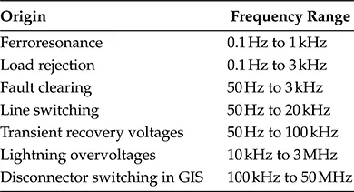
If a representation is already available for each frequency, the selection of the model may suppose an iterative procedure: the model must be selected based on the frequency range of the transients to be simulated; however, the frequency ranges of the test case are not usually known before performing the simulation. This task can be alleviated by looking into widely accepted classification tables. Table 1.1 shows a short list of common transient phenomena.
An important effort has been dedicated to clarify the main aspects to be considered when representing power components in transient simulations. Users of electromagnetic transient tools can nowadays obtain information on this field from several sources:
The document written by the CIGRE WG 33-02 covers the most important power components and proposes the representation of each component taking into account the frequency range of the transient phenomena to be simulated [2].
The fourth part of the IEC standard 60071 (TR 60071-4) provides modeling guidelines for insulation coordination studies when using numerical simulation, e.g., EMTP-like tools [3].
The documents produced by the Institute of Electrical and Electronics Engineers (IEEE) WG on modeling and analysis of system transients using digital programs and its task forces present modeling guidelines for several particular types of studies [4].
Table 1.2 provides a summary of modeling guidelines for the representation of the most important power components in transient simulations taking into account the frequency range.
The simulation of a transient phenomenon implies not only the selection of models but the selection of the system area that must be represented. Some rules to be considered in the simulation of electromagnetic transients when selecting models and the system area can be summarized as follows [5]:
TABLE 1.1
Origin and Frequency Ranges of Transients in Power Systems
TABLE 1.2
Modeling of Power Components for Transient Simulations
Select the system zone taking into account the frequency range of the transients; the higher the frequencies, the smaller the zone modeled.
Minimize the part of the system to be represented. An increased number of components does not necessarily mean increased accuracy, since there could be a higher probability of insufficient or wrong modeling. In addition, a very detailed representation of a system will usually require longer simulation time.
Implement an adequate representation of losses. Since their effect on maximum voltages and oscillation frequencies is limited, they do not play a critical role in many cases. There are, however, some cases (e.g., ferroresonance or capacitor bank switching) for which losses are critical to defining the magnitude of overvoltages.
Consider an idealized representation of some components if the system to be simulated is too complex. Such representation will facilitate the edition of the data file and simplify the analysis of simulation results.
Perform a sensitivity study if one or several parameters cannot be accurately determined. Results derived from such a sensitivity study will show what parameters are of concern.
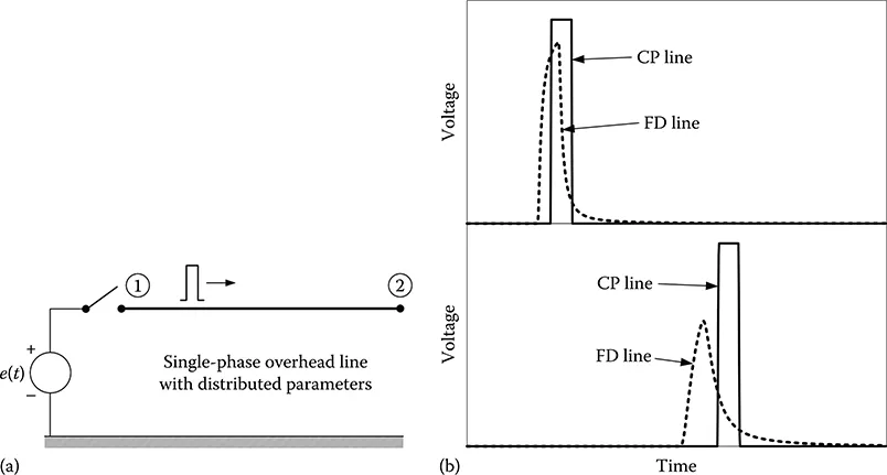
Figure 1.2 shows a test case used for illustrating the differences between simulation results from two different line models with distributed parameters: the lossless constant-parameter (CP) line and the lossy frequency-dependent (FD) line. Wave propagation along an overhead line is damped and the waveform is distorted when the FD-line model is used, while the wave propagates without any change if the line is assumed ideal (i.e., lossless), as expected. In addition the propagation velocity is higher with the FD-line model.
FIGURE 1.2
Comparative modeling of lines: FD and CP models. (a) Scheme of the test case; (b) wave propogation along the line.
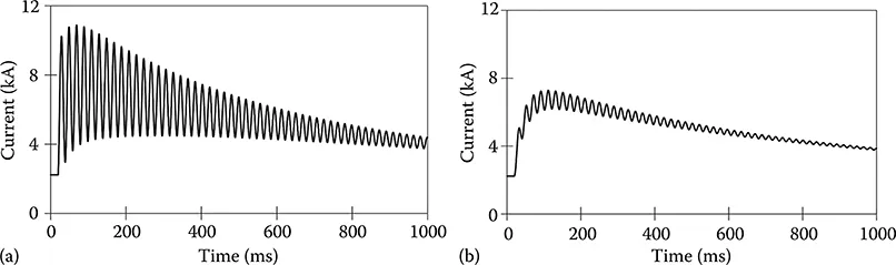
FIGURE 1.3
Field winding current in a synchronous generator during a three-phase short circuit. (a) Field current when coupling between the rotor d-axis circuits is assumed; (b) field current when coupling between the rotor d-axis circuits is neglected. (From Martinez, J.A. et al., IEEE Power Energy Mag., 3, 16, 2005. With permission.)
Frequency-dependent modeling can be crucial in some overvoltage studies; e.g., those related to lightning and switching transients. In breaker performance studies, since the breaker arc voltage excites all circuit frequencies, it might be important to apply frequency-dependent models even for substation bus-bar sections where the breaker effect is analyzed.
Figure 1.3 shows the field current in a synchronous generator during a three-phase short circuit at the armature terminals obtained with two different models. The first model assumes a coupling between the two rotor circuits located on the d-axis (field and damping windings), while this coupling has been neglected in the simulation of the second case. Although the differences are important, both modeling approaches can be acceptable if the main goal is to obtain the short circuit current in the armature windings or the deviation of the rotor angular velocity with respect to the synchronous velocity.
1.3 Parameter Determination
Given the different design and operation principles of the most important power components, various techniques can be used to analyze their behavior. The following paragraphs discuss the effects that have to be represented in mathematical models and what are the approaches that can be used to determine the parameters, without covering the determination of parameters needed to represent mechanical systems, control systems, or semiconductor models.
Basically, the mathematical model of a power component (e.g., line, cable, transformer, rotating machine) for electromagnetic transient analysis must represent the effects of electromagnetic fields and losses [1]:
Electr...