Dynamic programming (DP) and reinforcement learning (RL) are algorithmic methods for solving problems in which actions (decisions) are applied to a system over an extended period of time, in order to achieve a desired goal. DP methods require a model of the system’s behavior, whereas RL methods do not. The time variable is usually discrete and actions are taken at every discrete time step, leading to a sequential decision-making problem. The actions are taken in closed loop, which means that the outcome of earlier actions is monitored and taken into account when choosing new actions. Rewards are provided that evaluate the one-step decision-making performance, and the goal is to optimize the long-term performance, measured by the total reward accumulated over the course of interaction.
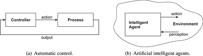
Such decision-making problems appear in a wide variety of fields, including automatic control, artificial intelligence, operations research, economics, and medicine. For instance, in automatic control, as shown in Figure 1.1(a), a controller receives output measurements from a process, and applies actions to this process in order to make its behavior satisfy certain requirements (Levine, 1996). In this context, DP and RL methods can be applied to solve optimal control problems, in which the behavior of the process is evaluated using a cost function that plays a similar role to the rewards. The decision maker is the controller, and the system is the controlled process.
FIGURE 1.1
Two application domains for dynamic programming and reinforcement learning.
In artificial intelligence, DP and RL are useful to obtain optimal behavior for intelligent agents, which, as shown in Figure 1.1(b), monitor their environment through perceptions and influence it by applying actions (Russell and Norvig, 2003). The decision maker is now the agent, and the system is the agent’s environment.
If a model of the system is available, DP methods can be applied. A key benefit of DP methods is that they make few assumptions on the system, which can generally be nonlinear and stochastic (Bertsekas, 2005a, 2007). This is in contrast to, e.g., classical techniques from automatic control, many of which require restrictive assumptions on the system, such as linearity or determinism. Moreover, many DP methods do not require an analytical expression of the model, but are able to work with a simulation model instead. Constructing a simulation model is often easier than deriving an analytical model, especially when the system behavior is stochastic.
However, sometimes a model of the system cannot be obtained at all, e.g., because the system is not fully known beforehand, is insufficiently understood, or obtaining a model is too costly. RL methods are helpful in this case, since they work using only data obtained from the system, without requiring a model of its behavior (Sutton and Barto, 1998). Offline RL methods are applicable if data can be obtained in advance. Online RL algorithms learn a solution by interacting with the system, and can therefore be applied even when data is not available in advance. For instance, intelligent agents are often placed in environments that are not fully known beforehand, which makes it impossible to obtain data in advance. Note that RL methods can, of course, also be applied when a model is available, simply by using the model instead of the real system to generate data.
In this book, we primarily adopt a control-theoretic point of view, and hence employ control-theoretical notation and terminology, and choose control systems as examples to illustrate the behavior of DP and RL algorithms. We nevertheless also exploit results from other fields, in particular the strong body of RL research from the field of artificial intelligence. Moreover, the methodology we describe is applicable to sequential decision problems in many other fields.
The remainder of this introductory chapter is organized as follows. In Section 1.1, an outline of the DP/RL problem and its solution is given. Section 1.2 then introduces the challenge of approximating the solution, which is a central topic of this book. Finally, in Section 1.3, the organization of the book is explained.
1.1 The dynamic programming and reinforcement learning problem
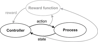
The main elements of the DP and RL problem, together with their flow of interaction, are represented in Figure 1.2: a controller interacts with a process by means of states and actions, and receives rewards according to a reward function. For the DP and RL algorithms considered in this book, an important requirement is the availability of a signal that completely describes the current state of the process (this requirement will be formalized in Chapter 2). This is why the process shown in Figure 1.2 outputs a state signal.
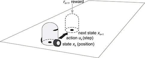
To clarify the meaning of the elements of Figure 1.2, we use a conceptual robotic navigation example. Autonomous mobile robotics is an application domain where automatic control and artificial intelligence meet in a natural way, since a mobile robot and its environment comprise a process that must be controlled, while the robot is also an artificial agent that must accomplish a task in its environment. Figure 1.3 presents the navigation example, in which the robot shown in the bottom region must navigate to the goal on the top-right, while avoiding the obstacle represented by a gray block. (For instance, in the field of rescue robotics, the goal might represent the location of a victim to be rescued.) The controller is the robot’s software, and the process consists of the robot’s environment (the surface on which it moves, the obstacle, and the goal) together with the body of the robot itself. It should be emphasized that in DP and RL, the physical body of the decision-making entity (if it has one), its sensors and actuators, as well as any fixed lower-level controllers, are all considered to be a part of the process, whereas the controller is taken to be only the decision-making algorithm.
FIGURE 1.2
The elements of DP and RL and their flow of interaction. The elements related to the reward are depicted in gray.
FIGURE 1.3
A robotic navigation example. An example transition is also shown, in which the current and next states are indicated by black dots, the action by a black arrow, and the reward by a gray arrow. The dotted silhouette represents the robot in the next state.
In the navigation example, the state is the position of the robot on the surface, given, e.g., in Cartesian coordinates, and the action is a step taken by the robot, similarly given in Cartesian coordinates. As a result of taking a step from the current position, the next position is obtained, according to a transition function. In this example, because both the positions and steps are represented in Cartesian coordinates, the transitions are most often additive: the next position is the sum of the current position and the step taken. More complicated transitions are obtained if the robot collides with the obstacle. Note that for simplicity, most of the dynamics of the robot, such as the motion of the wheels, have not been taken into account here. For instance, if the wheels can slip on the surface, the transitions become stochastic, in which case the next state is a random variable.
The quality of every transition is measured by a reward, generated according to the reward function. For instance, the reward could have a positive value such as 10 if the robot reaches the goal, a negative value such as −1, representing a penalty, if the robot collides with the obstacle, and a neutral value of 0 for any other transition. Alternatively, more informative rewards could be constructed, using, e.g., the distances to the goal and to the obstacle.
The behavior of the controller is dictated by its policy: a mapping from states into actions, which indicates what action (step) should be tak...