Understanding Econometrics

Jon Stewart

• Publisher: Taylor & Francis
• Year: 2018
• Print ISBN: 9780815350149
• eBook ISBN: 9781351140386
• Edition: 1
• Topic: Business
• Subtopic: Business General
• Index: Business

Originally published in 1976 and with second edition published in 1984. This book established itself as the first genuinely introductory text on econometric methods, assuming no formal background on the part of the reader. The second edition maintains this distinctive feature. Fundamental concepts are carefully explained and, where possible, techniques are developed by verbal reasoning rather than formal proof. It provides all the material for a basic course. and is also ideal for a student working alone. Very little knowledge of maths and statistics is assumed, and the logic of statistical method is carefully stated. There are numerous exercises, designed to help the student assess individual progress. Methods are described with computer solutions in mind and the author shows how a variety of different calculations can be performed with relatively simple programs. This new edition also includes much new material - statistical tables are now included and their use carefully explained.

1 Introduction

1.1 The nature of econometrics

Econometrics is a discipline embracing aspects of methodology from economics, mathematics and statistics. The econometrician is simply an economist who, in trying to understand the working of economic systems, makes use of techniques which are based primarily on the methodology of statistics and which are often communicated in the language of mathematics. This formal background to the subject is sometimes a deterrent to those who would like to understand the nature of econometrics, and this book represents an attempt to explain how and why econometric methods are used in a way which does not assume that the reader is already familiar with the mathematical and statistical concepts involved. Although the ideas introduced are precise and do have to be carefully used, formal derivation and proof is not always necessary and an explanation of why a particular result is likely to hold can often provide an adequate alternative.

1.2 Economic models

Before any progress can be made, it is necessary to understand exactly what is meant by an economic model. Economic systems are undoubtedly complex, and the idea of using a model arises because of this complexity. A model is an abstraction from reality, drawn in such a way as to reveal the major features of the system. Clearly, there can be ‘good’ and ‘bad’ models. If the abstraction is taken too far, the model may have little to say about the corresponding real system. If, on the other hand, the abstraction is not taken far enough, the model may be so complicated that one is unable to isolate those aspects of the real system that are of crucial importance.

Models exist in many forms. The analysis of any system must be based on a model, but the model need not necessarily be explicit. Economic journalism provides many examples of analysis which is obviously based on a set of assumptions — sometimes explicit, often not so — which represent an underlying model. It is clearly advantageous to those wishing to evaluate the analysis if the model can be given some explicit form.

The models with which the econometrician is typically concerned are expressed in mathematical form, but this is not true of explicit models in general or of economic models in particular. For example, a diagram showing the flows of goods, services and finance in the economy is a model. However, a model must be appropriate to the questions which the economist wishes to ask and, if he is concerned about the relationships between the flows, the flow diagram is unlikely to be sufficient on its own. In this case, the level of abstraction is taken too far.

The discussion in the remainder of this chapter is based largely on the example of a postulated relationship between consumers’ expenditure and personal disposable income at the macroeconomic level. The assertion that such a relationship should exist is a model, but one which is insufficiently precise to answer questions concerning the magnitude of the changes in consumption that occur as a response to changes in income. To make progress, the relationship must be given some explicit form. One way in which this can be done is to make the relationship as simple as possible, until such time as there is evidence, from observation of a real system, that the simple form is inadequate. This is a useful approach for an introductory text, but the reader should not jump to the conclusion that all modelling exercises start with very simple relationships or that the ability to reproduce observed behaviour is the only test of model adequacy that one might use.

1.3 A simple model

Suppose that, for a hypothetical economy, there exists a relationship between consumers’ expenditure C and personal disposable income D that can be expressed as

C=50+0⋅8D(1.3.1)

In this equation, C and D are variables which can take different values at different points of observation of the economic system. The numbers 50 and 0*8 are constants. To fix ideas, suppose that consumption and income flows were observed for each of two time periods. Then, whereas consumption and income would generally take distinct values in each period, the existence of a fixed relationship would imply that the numbers 50 and 0*8 remain the same. Although the values of the variables change, the relationship between the variables does not.

The graph corresponding to equation 1.3.1. is shown in Figure 1.

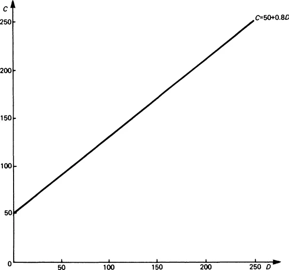
Figure 1

It can be seen from the graph that the equation represents a straight line. If consumer behaviour in the (hypothetical) economy is described by this equation, each pair of consumption and income values represents a single point which would He on the straight line. A more general representation for a straight line or linear relationship between C and D is:

C⁢=α+βD(1.3.2)

where α and β are described as parameters of the relationship. In our hypothetical economy, α = 50 and β = 0·8. In a second case there might again be a linear relationship, but with different parameter values.

Parameter α is called the intercept and parameter β the slope. The intercept represents the value of consumption which, according to the equation, would hold if income were zero. The slope represents the change in consumption resulting from a unit change in income. If this is not obvious, use equation 1.3.1 with income levels of 0 and 1:

C=50+0⋅8(0)=50C=50+0⋅8(1)=50⋅8

The increase in consumption for a unit increase in income is thus 0·8, and this is the value of β in the hypothetical economy. Because the relationship is linear, the effect of a unit change in income is always the same, irrespective of the point from which the unit change takes place.

If equation 1.3.2 is interpreted as determining the level of consumption for a given level of income, consumption is said to be the dependent variable and income is said to be the explanatory variable. In economic terminology the relationship would be described as a linear version of the consumption function, and β would be the marginal propensity to consume. The marginal propensity to consume is simply the slope of the consumption function, but it is important to realize that it is only in the case of a linear function that the slope is a constant and does not depend on the values taken by C or D. The graph corresponding to a nonlinear relationship would be a curve rather than a straight line and, in the case of a curve, the slope does change as the values of the variables change.

In what follows we shall concentrate largely on linear relationships, and it is important, in several distinct contexts, to be able to recognize when a given relationship is linear. The equation

5C=250⁢+4D

does represent a linear relationship, because division by 5 on both sides gives

C⁢=50+0⋅8D

which is in the standard linear form. In c...

Table of contents

• Cover
• Half Title
• Title Page
• Copyright Page
• Contents
• Preface to the first edition
• Preface to the second edition
• 1 Introduction
• 2 The two variable linear model
• 3 The linear model with further explanatory variables
• 4 Alternative disturbance specifications
• 5 Distributed lags and dynamic economic models
• 6 Simultaneous equation models
• Suggestions for further reading
• Statistical tables
• Solutions to exercises
• Index