Remote and Robotic Investigations of the Solar System

C.R. Kitchin

• Publisher: CRC Press
• Year: 2017
• eBook ISBN:
  9781351255462
• Subtopic: Science Research & Methodology

Interest in and knowledge of the techniques utilised to investigate our solar system has been growing rapidly for decades and has now reached a stage of maturity. Therefore, the time has now arrived for a book that provides a cohesive and coherent account of how we have obtained our present knowledge of solar system objects, not including the Sun.

Remote and Robotic Investigations of the Solar System covers all aspects of solar system observations: the instruments, their theory, and their practical use both on Earth and in space. It explores the state-of-the-art telescopes, cameras, spacecraft and instruments used to analyse the interiors, surfaces, atmospheres and radiation belts of solar system objects, in addition to radio waves, gamma rays, cosmic rays and neutrinos. This book would be ideal for university students undertaking physical science subjects and professionals working in the field, in addition to amateur astronomers and anyone interested in learning more about our local astronomical neighbours.

I

The Detection and Investigation of Solar System Objects via Electromagnetic Radiation

CHAPTER 1

The Extended Optical Region

1.1 INTRODUCTION

In this first part, the aim is to describe, explain and discuss the ways in which our knowledge of the solar system and its contents has been enlarged and enhanced by remote and robotic investigations utilising the photons emitted or reflected from solar system objects. Later parts will deal with more direct and interactive investigations.

Readers of this book are likely to be familiar with the dual wave-particle nature of electromagnetic (e-m) radiation. A reminder of what this implies for the design of instrumentation, etc. however may not come amiss – thus the wave nature of light enables a telescope lens or mirror to focus a beam of (wave) radiation into an image, whilst the detector, in most cases, will utilise the particle nature of light to pick up individual photons.

When behaving as a wave, e-m radiation is described by its frequency (ν or f^*) and wavelength (λ) and, in a vacuum, the two quantities are related to the velocity of light in a vacuum (c) by

$$\lambda \nu =c$$(1.1)

The e-m radiation in its particle manifestation is described by the energy of the individual photons (quanta) that are involved. The wave and particle descriptions are linked by the Planck formula

$$E=h\nu$$(1.2)

where h is Planck’s constant (6.62607 × 10⁻³⁴ m² kg s⁻¹) and E is the photon’s energy.

Conversion between the frequency, wavelength and energy of e-m radiation is often needed and the formulae

$$\begin{array}{lllll}\text{Frequency}\left(\text{Hz}\right)\hfill & \approx \hfill & 3.00\times {10}^8\hfill & ÷\hfill & \text{Wavelength}\left(\text{m}\right)\hfill \\ \hfill & \approx \hfill & 1.50\times {10}^{33}\hfill & \times \hfill & \text{Energy}\left(\text{J}\right)\hfill \\ \hfill & \approx \hfill & 2.40\times {10}^{14}\hfill & \times \hfill & \text{Energy}\left(\text{eV}\right)\hfill \end{array}$$(1.3)

$$\begin{array}{lllll}\text{Wavelength}\left(\text{m}\right)\hfill & \approx \hfill & 3.00\times {10}^8\hfill & ÷\hfill & \text{Frequency}\left(\text{Hz}\right)\hfill \\ \hfill & \approx \hfill & 2.00\times {10}^{-25}\hfill & ÷\hfill & \text{Energy}\left(\text{J}\right)\hfill \\ \hfill & \approx \hfill & 1.25\times {10}^{-6}\hfill & ÷\hfill & \text{Energy}\left(\text{eV}\right)\hfill \end{array}$$(1.4)

$$\begin{array}{lllll}\text{Energy}\left(\text{J}\right)\hfill & \approx \hfill & 1.60\times {10}^{-19}\hfill & \times \hfill & \text{Energy}\left(\text{eV}\right)\hfill \\ \hfill & \approx \hfill & 6.66\times {10}^{-34}\hfill & \times \hfill & \text{Frequency}\left(\text{Hz}\right)\hfill \\ \hfill & \approx \hfill & 2.00\times {10}^{-25}\hfill & ÷\hfill & \text{Wavelength}\left(\text{m}\right)\hfill \end{array}$$(1.5)

$$\begin{array}{lllll}\text{Energy}\left(\text{eV}\right)\hfill & \approx \hfill & 6.24\times {10}^{-18}\hfill & \times \hfill & \text{Energy}\left(\text{J}\right)\hfill \\ \hfill & \approx \hfill & 4.16\times {10}^{-15}\hfill & \times \hfill & \text{Frequency}\left(\text{Hz}\right)\hfill \\ \hfill & \approx \hfill & 1.25\times {10}^{-6}\hfill & ÷\hfill & \text{Wavelength}\left(\text{m}\right)\hfill \end{array}$$(1.6)

may be found useful (where the quantities are in the units usually used).

The e-m spectrum thus theoretically ranges from zero frequency or energy (infinite wavelength) to infinite frequency or energy (zero wavelength). It is customarily subdivided, in terms of its frequency, into the regions:^*

0 ↔ Extremely low frequency (ELF) ↔ Radio ↔ Microwave
↔ Far infrared (FIR^†) ↔ Medium infrared (MIR) ↔ Near infrared (NIR) ↔ Visible^‡
↔ Ultraviolet ↔ Soft x-rays ↔ Hard x-rays ↔ γ rays ↔ ∞

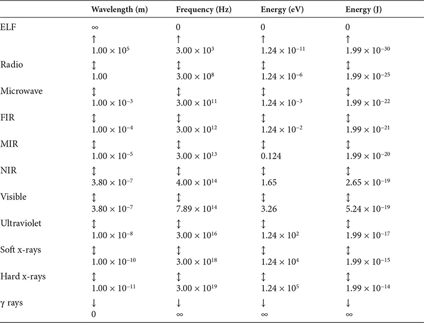
The approximate extents of these regions are shown in Table 1.1 together with conversions between wavelength, frequency and energy for quick reference.

E-m radiation is generally, but by no means always, discussed in terms of its frequency at low energies (ELF, radio, microwave regions), by its wavelength in the intermediate region (infrared [IR], visible and ultraviolet [UV] regions) and by the photon energy in the x-ray and γ ray regions. This practice is mainly historical in origin, but remains convenient in that the numbers thus being used have relatively small powers of ten in their expressions.

A reminder may also be useful that e-m radiation interacts with matter in different ways depending upon its energy (particle character)/frequency (wave character). Thus, the main interactions are:

• ELF and radio radiation – direct induction of electric currents, synchrotron and free-free emissions and absorptions
• Microwave and Infrared – molecular rotational and vibrational emissions and absorptions
• Optical – interactions with the outer electrons of atoms, ions and molecules
• UV and x-ray – interactions with the inner electrons of atoms and ions, ionisation and recombination
• X-ray and γ rays – interactions directly with nuclei

TABLE 1.1 The Regions of the e-m Spectrum and the Interrelationships between Frequency, Wavelength and Photon Energy

Thermal radiation can be emitted by materials at any temperature when their constituent atoms or molecules undergo changes of velocity during their interactions with other nearby atoms or molecules. The change in velocity results in bremsstrahlung^* radiation. In liquids and gases, the particles are free to move around. In solids, the particles are more or less fixed in place, but vibrate about their mean positions within the material so that the individual radiation patterns have a dipole nature. Thermal radiation’s spectrum^* is described by the Planck equation and its emissions peak at a wavelength or frequency for a particular temperature given by Wien’s displacement law.

Planck equation:

$$I\left(\nu ,T\right)\text{d}\nu =\frac{2h{\nu }^3{\mu }^2}{c^2\left(e^{h\nu /kT}-1\right)}$$(1.7)

$$I\left(\lambda ,T\right)\text{d}\lambda =\frac{2h{c}^2{\mu }^2}{{\lambda }^5\left(e^{h\nu /\lambda kT}-1\right)}$$(1.8)

and

$$I\left(\nu ,T\right)\text{d}\nu =I\left(\lambda ,T\right)\text{d}\lambda$$(1.9)

where I(ν,T) and I(λ,T) are the thermal radiation intensities at temperature T and in terms of frequency and wavelength, respectively, and μ is the refractive index of the material forming the transmission medium (equal to 1 for a vacuum).

Wien’s displacement law:

$${\lambda }_{\text{Max}}=\frac{2.898\times {10}^{-3}}{T}m$$(1.10)

$${\nu }_{\text{Max}}=5.879\times {10}^{10}T\text{Hz}$$(1.11)

where λ_Max and ν_Max are the wavelength and frequency of the maximum thermal emission per unit wavelength and unit frequency intervals.^†

Measurements of e-m radiation can, theoretically, determine its frequency (or wavelength or photon energy), its intensity at a particular frequency (and also the variation of its intensity as the frequency changes – i.e. the spectrum), its variation in intensity in one, two or three dimensions (i.e. the direction of its sources/imaging), its state of polarization and its phase. Generally, only at low frequencies can all these properties of radiation be determined and at the highest frequencies, measurements are limited largely to determining the radiation’s intensity and direction.

Particularly for the spacecraft-borne instrumentation used for studying the objects within the solar system, the main observing region of the spectrum ranges from microwaves to soft x-rays. Over much of this region instruments’ operating principles are clearly related to each other, although the details vary. We shall therefore start by looking at the instrumentation used over the MIR to UV parts of the spectrum before going on to consider instruments operating at lower or higher frequencies. Since, as already mentioned, the term ‘optical region’ is generally used for the NIR, visible and near UV regions, it is convenient to use the term ‘extended optical region’ (EOR), to include the MIR and far UV regions as well.

1.2 TELESCOPES AND CAMERAS

Most people find that the direct images of objects, whether black and white, colour or false colour, are the most vivid and impressive results from spacecraft solar system missions. The implications of such images may normally be understood immediately, without (or without much) specialist training. From a scientific point of view, images contain a wealth of information and form an invaluable reference archive even after they have been used for their primary purpose(s). Obtaining images over the EOR customarily involves using telescopes – or since the instruments do not use eyepieces, what should more properly be called cameras.

Apart from the lack of an eyepiece, the cameras on spacecraft are often identical in their designs to terrestrial telescopes, or are minor variants of such designs. Both refracting (lens-based, dioptric) and reflecting (mirror-based, catoptric) instruments are in use, with the latter being the more common. There are also some custom-built optical systems that have been designed (usually) because of constraints on mass or size required within a particular spacecraft.

Almost all of these camera designs may include additional optics to fold the light beam in order to shorten the instrument’s length or to direct the image to a convenient place. Most cameras have interchangeable filters to enable images to be obtained within different parts of the spectrum and/or be multipurpose instruments obtaining direct images or spectra (Section 1.3) or both simultaneously.

The reader is assumed to be familiar with the basics of the optics of light – laws such as those of reflection and refraction and terms such as focal plane, field of view, focal length, focal ratio, etc. The basic principles of usual designs of cameras (telescopes) are likely to be familiar to most readers of this book, but if not, Appendix A lists various sources suitable for background reading. Here just a brief summary of the main designs is given with examples of their use in actual missions.

1.2.1 Reflecting Cameras

Some cameras are based just upon a single concave parabolic mirror with the detector or detector array placed at its focus – a system known as a prime focus instrument when used for terrestrial telescopes (Figure 1.1a). Subsidiary lenses or mirrors will generally be needed to correct the aberrations^* inherent in a simple parabolic mirror, providing a wider, sharply focussed, field of view. The Cassegrain design (Figure 1.1b) uses a concave parabolic primary mirror and a convex hyperbolic secondary mirror. The closely related Ritchey–Chrétien instruments have a wider field of sharp focus than a similar Cassegrain and use a concave hyperbolic primary mirror and a convex hyperbolic secondary mirror. Some Gregorian-based designs (Figure 1.1c) are also to b...

Table of contents

• Cover
• Half Title
• Title Page
• Copyright Page
• Contents
• Preface
• Part I The Detection and Investigation of Solar System Objects via Electromagnetic Radiation
• Part II The Detection and Investigation of Sub-Atomic, Atomic and Molecular Particles
• Part III Direct Sampling and Other Investigative Methods
• Appendix A: Bibliography
• Appendix B: Timeline of Solar System Investigations
• Appendix C: Details of the Spacecraft, Rockets, Observatories and Other Missions Mentioned in this Book
• Appendix D: Data and Units
• Appendix E: Abbreviations and Acronyms
• Index