Practical Longitudinal Data Analysis

David J. Hand, Martin J. Crowder

• Publisher: Routledge
• Year: 2017
• Print ISBN: 9780367833961
• eBook ISBN: 9781351422659
• Topic: Mathematics
• Subtopic: Probability & Statistics
• Index: Mathematics

This text describes regression-based approaches to analyzing longitudinal and repeated measures data. It emphasizes statistical models, discusses the relationships between different approaches, and uses real data to illustrate practical applications. It uses commercially available software when it exists and illustrates the program code and output. The data appendix provides many real data sets-beyond those used for the examples-which can serve as the basis for exercises.

CHAPTER 1

Introduction

1.1 Introduction

One of the attractive features of repeated measures data is that (for numerical data, at least) they can be displayed in a graphical plot which is readily interpretable, without requiring a great effort. Table A.1 (in Appendix A) shows measurements of the body weights of rats on three different diets, measured on 11 occasions. Figure 1.1 shows a plot of change in weight over time for the rats on diet 1. The horizontal axis shows time (in days) and the vertical axis weight (in grams). The values for individual rats are shown connected by straight lines.

We can clearly see that, in general, the rats gain weight with passing time (the overall positive slope of the plots) and that, although there is some irregularity, all of the rats follow the same basic pattern. There seems to be no suggestion that the variance of the weights increases with time. We can also see that one of the rats is an outlier, beginning with a low weight and remaining low – although also following a path more or less parallel to the others.

For none of this does one need any training in interpreting the plots.

But, of course, this does not go far enough. We want to be able to make more than general statements summarizing the apparent behaviour of the units being studied. We want to quantify this behaviour, we want to describe it accurately, and we want to compare the behaviour of different groups of units. This book describes methods for doing these things.

Before going into detail, let us define a few of the basic terms and some of the notation we shall use. The units being studied, each of which is measured on several occasions (or, conceivably, under several conditions) will be called (experimental) units, individuals or, sometimes, subjects. They will be measured at several occasions or times. Together the results of these measurements will form a response profile (or curve or, sometimes, trend) for each unit. And our aim is to model the mean response profiles in the groups. (The word ‘clustered’ is sometimes used for repeated measures data. However, with its usual English meaning it would seem to be more appropriate for groups of observations in classical split plots than for strings of observations taken over a time period.)

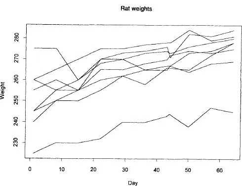
Figure 1.1 Plots showing the change in rat weights over time. The data are given in Crowder and Hand (1990, Table 2.4), and are reproduced in Table A.1.

The fact that we are discussing means will alert the reader to the main distinction between time series and the subject matter of this text. Instead of the single (long) series of observations which characterizes a time series, we shall assume that we have several (perhaps many) relatively short series of observations, one for each unit. The existence of multiple series gives us the advantage that we can more readily test (rather than assume) particular structures for the covariance matrix relating observations at subsequent times.

A word or two about notation is also appropriate. As in our previous book, a consistent notation will be used throughout. Thus, y_ij will denote the jth measurement made on the ith individual. Its mean is ${\mu }_{ij}=E\left(y_{ij}\right)$, its variance is ${\sigma }_{ij}^2=\mathrm{var}(y_{ij})$, and it will often be accompanied by a vector x_ij of explanatory variables. The number of individuals in the sample will usually be n, the number of measures made on individual i will be p, or maybe p_i when these differ, and the dimension of x_ij will usually be q. The set of measures $y_{ij}\left(j=1,\dots ,p\right)$ will often be collected into a p × 1 vector y_i, with mean vector μ_i and covariance matrix Σ_i.

Clearly, the problem we are addressing is intrinsically multivariate. However, it involves a restricted form of multivariate data. Three observations are of particular interest here. First, the same ‘thing’ is being measured at each time – so that the measurements are commensurate. This is not true of general multivariate data, where one variable might be height, another weight, and so on.

Second, the measures are typically taken at selected occasions on an underlying (time) continuum. Sometimes the individuals are measured on different occasions or on different numbers of occasions. This may complicate the analysis in practice, but it does not alter it in principle: the measurements are simply an attempt to get at the underlying continuous curve of change over time (or of probability of occupying a particular state in discrete cases). This is quite different from the general multivariate case, where there is no underlying continuum.

Third, the sequential nature of the observations means that particular kinds of covariance structures are likely to arise, unlike more general multivariate situations, where there may be few or no indications of the structure.

The inherent dependence, or the possibility of dependence, that is associated with longitudinal data introduces extra complications into the analysis. No longer can we rely on the simplifying properties arising from data which are independently and identically distributed. To yield conclusions in which we can have confidence, we must somehow take the possible dependence into account. Nevertheless, the simplicity of methods of analysis which assume independence is attractive. It is therefore hardly surprising that researchers have explored methods which modify the problem so that independence-based approaches can be used. In the next two sections of this chapter we describe two such methods. The first analyses each time separately, and we do not recommend this approach for several reasons. The second summarizes the profiles and works with these summaries. Section 1.4 summarizes the more sophisticated methods described in later chapters.

Before we leave this introductory section, however, to give the reader a flavour of the rich variety of problems which can arise in a longitudinal context, we show, in Figs 1.2 to 1.7, a series of plots of the response profiles from different problems. (Necessarily, these plots only show data which have arisen from numerical measurements. Discrete data yield another entire class of possible kinds of problem.) These figures illustrate the range of profiles which can arise, and the sorts of structures one might look for.

1.2 Comparisons at each time

As we have pointed out above, the distinctive feature of longitudinal data is that the observations on a particular individual at each time will not, in general, be independent. Somehow this has to be taken into account in any analysis – unless the particular circumstances of a problem mean that a justification for not making allowance for it can be found (Chapter 3). One approach which has been common in the past, and which has the merit of simplicity, is to analyse each time separately. Of course, this is restricted to those situations where all of the individuals are measured at the same time (or where the times can be grouped so that they are regarded as simultaneous). Groups can be compared at each time using t-tests, standard univariate analysis of variance, or nonparametric groups comparisons as appropriate.

While this approach may be attractive because of its simplicity, it does have some serious deficiencies. The only way it can shed light on the change of treatment effects with time is by a comparison of the separate analyses. A similar comparison could be made using independent groups at each time. At best, what can be obtained are statements about the change of averages – and not about the average of changes. The two might be quite different and, as we have remarked, it is typically the latter which is of interest. The advantages of undertaking a longitudinal study have been lost. Moreover, the tests are not independent, since the data have arisen from the same experimental units. The fact that one particular group scores significantly more highly than another on several occasions is not as strong evidence for the superiority of that group as would be the case if the tests were independent. (This is further complicated by the fact that several tests have been conducted.) Sometimes, also, the tests are compared with a view to deciding ‘when’ an effect occurs – the time being identified as that at which a significant difference first arises. This is, of course, usually meaningless because of the continuous nature of changes.

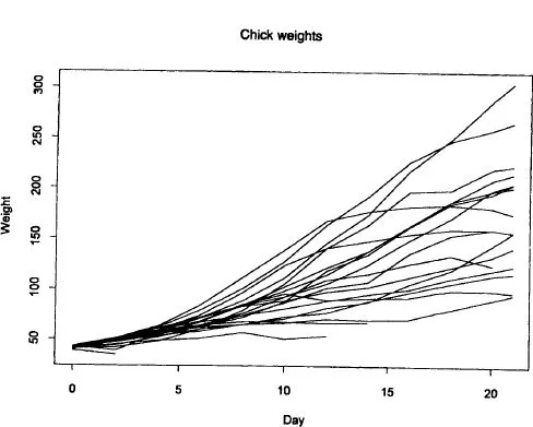
Figure 1.2 Body weights of 20 chicks on a normal diet, measured on alternate days. The data are the first 20 rows of Table A.2. The fan shape, showing variance increasing with time, is typical of growth curves.

In summary, the approach based on testing the results at each time separately is typically invalid. More sophisticated methods, which take account of the relationships between observations at different times, need to be used. This book describes such methods.

1.3 Response feature analysis

Section 1.2 described a method of analysis which has been common in the past (though we would like to think it is less so nowadays since powerful computer software has become available which permits more valid analyses to be readily performed). This section describes another simple method which is quite common, and which is statistically valid. Its main weakness is that it may be not very powerful.

This text describes models which can be fitted to sequences of responses over time. Important aspects of the process generating the data are identified and these are used to produce a well-fitting model. Often, however, researchers’ interests lie in a particular aspect of the change over time. For example, they might want to know the peak value achieved after administration of some treatment, the time taken to return to some baseline value, the difference between average post-treatment and average pre-treatment scores, the area under some response curve, or simply the slope showing rate of change over time. We call such an aspect of the profile a response feature beause it summarizes some aspect of the response over time, and the approach to analysis which concentrates solely on such features, response feature analysis.

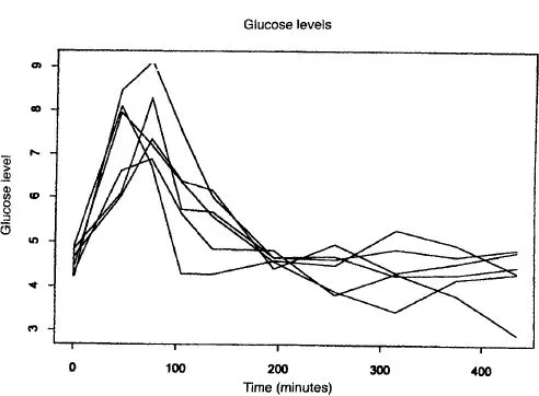
Figure 1.3 Blood glucose levels following a meal taken at time 15 minutes. The data are given in Table A.3. The response builds up to a peak soon after the meal, and then gradually decays.

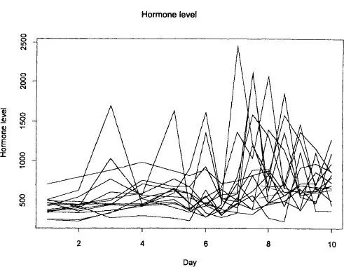
Figure 1.4 Luteinizing hormone levels in non-suckling cows (ng ml⁻¹ × 1000), listed in Table A.4, with cow number 7 removed as it has a very large score at 9.5 days. Some of these profiles show marked variability: while we may draw conclusions about the mean profile, we must bear in mind that individuals may depart substantially from this.

The approach has several merits. It is easy to understand and explain, and it leads to a simple univariate analysis – the vector of measurements on each subject is reduced to a single summarizing score, focusing on the information of particular interest. Moreover, the summarizing features can often be calculated even if subjects have different numbers of measurements and are measured at different times. This is a powerful advantage since missing data are common in studies which extend over time. The method focuses attention on the shapes of curves for the individuals – and not on the curve through the means at each time, which might be quite different. (This is where the method described in section 1.2 failed.)

The chi...

Table of contents

• Cover
• Half Title
• Title Page
• Copyright Page
• Table of Contents
• Preface
• 1. Introduction
• Part One: Normal Error Distributions
• Part Two: Non-normal Error Distributions
• Part Three: Comparisons of Methods
• Appendix A The data sets used in the examples
• Appendix B Extra data sets
• References
• Author index
• Subject index