Statistical Models in S

T.J. Hastie

• Publisher: Routledge
• Year: 2017
• eBook ISBN: 9781351414227
• Topic: Mathematics
• Subtopic: Probability & Statistics
• Index: Mathematics

Statistical Models in S extends the S language to fit and analyze a variety of statistical models, including analysis of variance, generalized linear models, additive models, local regression, and tree-based models. The contributions of the ten authors-most of whom work in the statistics research department at AT&T Bell Laboratories-represent results of research in both the computational and statistical aspects of modeling data.

Chapter 1

An Appetizer

John M. Chambers
Trevor J. Hastie

This book is about data and statistical models that try to explain data. It is an enormous topic, and we will discuss many aspects of it. Before getting down to details, however, we present an appetizer to give the flavor of the large meal to come. The rest of this chapter presents an example of models used in the analysis of some data. The data are “real,” the analysis provided insight, and the results were relevant to the application. We think the story is interesting. Besides that, it should give you a feeling for the style of the book, for our approach to statistical models, and for how you can use the software we are presenting. Don’t be concerned if details are not explained here; all should become clear later on.

1.1 A Manufacturing Experiment

In 1988 an experiment was designed and implemented at one of AT&T’s factories to investigate alternatives in the “wave-soldering” procedure for mounting electronic components on printed circuit boards. The experiment varied a number of factors relevant to the engineering of wave-soldering. The response, measured by eye, is a count of the number of visible solder skips for a board soldered under a particular choice of levels for the experimental factors. The S object containing the design, solder .balance, consists of 720 measurements of the response skips in a balanced subset of all the experimental runs, with the corresponding values for five experimental factors. Here is a sample of 10 runs from the total of 720.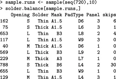

We can also summarize each of the factors and the response:

The physical and statistical background to these experiments is fascinating, but a bit beyond our scope. The paper by Comizzoli, Landwehr, and Sinclair (1990) gives a readable, general discussion. Here is a brief description of the factors:

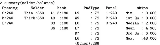
Opening: amount of clearance around the mounting pad;

Solder: amount of solder;

Mask: type and thickness of the material used for the solder mask;

PadType: the geometry and size of the mounting pad; and

Panel: each board was divided into three panels, with three runs on a board.

Much useful information about the experiment can be seen without any formal modeling, particularly using plots. Figure 1.1, produced by the expression

plot (solder. balance)

is a graphical summary of the relationship between the response and the factors, showing the mean value of the response at each level of each factor. It is immediately obvious that the factor Opening has a very strong effect on the response: for levels M and L, only about two skips were seen on average, while level S produced about six times as many. If you guessed that the levels stand for small, medium, and large openings, you were right, and the obvious conclusion that the chosen small opening was too small (produced too many skips) was an important result of the experiment.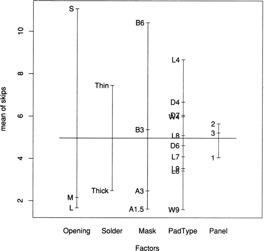

Figure 1.1: A plot of the mean of skips at each of the levels of the factors in the solder experiment. The plot is produced by the expression plot (solder .balance).

A more detailed preliminary plot can be obtained using plot.factor (), which produces a separate boxplot for each factor:

plot.factor(skips ~ Opening + Mask)

We have selected two of the factors for this plot, shown in Figure 1.2, and they both exhibit the same behavior: the variance of the response increases with the mean. The response values are counts, and therefore are likely to exhibit such behavior, since counts are often well described by a Poisson distribution.

Figure 1.2: A factor plot gives a separate boxplot of skips at each of the levels of the factors in the solder experiment. The left panel shows how the distribution of skips varies with the levels of Opening, and the right shows similarly how it varies with levels of mask.

1.2 Models for the Experimental Results

Now let’s start the process of modeling the data. We can, and will, represent the Poisson behavior mentioned above. To begin, however, we will use as a response sqrt (skips), since square roots often produce a good approximation to an additive model with normal errors when applied to counts. Since the data form a balanced design, the classical analysis of variance model is attractive. As a first attempt, we fit all the factors, main effects only. This model is described by the formula

sqrt (skips) ~.

where the saves us writing out all the factor names. We read as “is modeled as”; it separates the response from the predictors. The fit is computed by

> fit1 <- aov(sqrt(skips) ~ ., data = solder.balance)

The object fit1 represents the fitted model. As with any S object, typing its name invokes a method for printing it:

> fitl

Call:

aov(formula = sqrt(skips) ~ Opening + Solder + Mask + PadType +

Panel, data = solder.balance)

Residual standard error: 0.83806

Estimated effects are balanced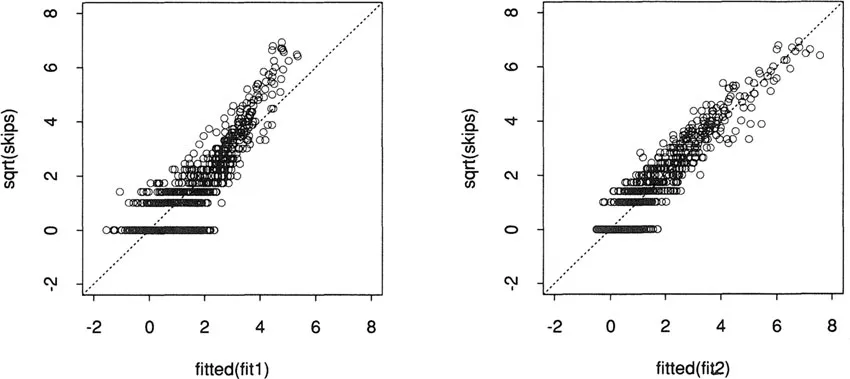

Figure 1.3: The left panel shows the observed values for the square root of skips, plotted against the fitted values from the main-effects model. The dotted line represents a perfect fit. The fit seems poor in the upper range. The right panel is the same plot for the model having main effects and all second-order interactions. The fit appears acceptable.

Once again, plots give more information. The expression

plot(fitted(fit1), sqrt(skips))

shown on the left in Figure 1.3, plots the observed skips against the fitted values, both on the square-root scale. The square-root transformation has apparently done a fair job of stabilizing the variance. However, the main-effects model consistently underestimates the large values of skips. With 702 degrees of freedom for residuals, we can afford to try a more extensive model. The formula

sqrt (skips) ~ . ^2

describes a model that includes all main effects and all second-order interactions. We fit this model next:

fit2 <- aov(sqrt(skips) ~ .^2, solder. balance)

Instead of printing the fitted object, we produce a statistical summary of the model using standard statistical assumptions, in this case an analysis of variance table as shown in Table 1.1, with mean squares and F-statistic values.

Table 1.1: An analysis of variance table for the model fit2, including all main effects and second-order interactions. The columns give degrees of freedom, sums of squares, mean squares, F statistics, and their tail probabilities, nearly all zero here because of the very large number of observations.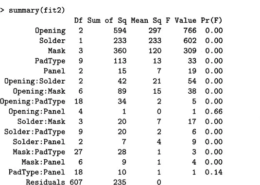

The function summary () is generic, in that it automatically behaves differently, according to the class of its argument. In this case fit2 has class “aov” and so a particular method for summarizing aov objects is automatically used. The earlier use of summary () produced a result appropriate for data. frame objects. The modeling software abounds with generic functions; besides summary(), others include plot(), predict(), print(), and update().

The fitted values are plotted in the right panel of Figure 1.3, and the improvement is clear. Of course, we really expect an improvement; including all the pairwise interactio...

Table of contents

• Cover
• Half Title
• Title Page
• Copyright Page
• Table of Contents
• 1 An Appetizer
• 2 Statistical Models
• 3 Data for Models John M. Chambers
• 4 Linear Models
• 5 Analysis of Variance; Designed Experiments
• 6 Generalized Linear Models
• 7 Generalized Additive Models
• 8 Local Regression Models
• 9 Tree-Based Models
• 10 Nonlinear Models
• A Classes and Methods: Object-oriented Programming in S John M. Chambers
• B S Functions and Classes
• References
• Index