A Beginner's Guide to Image Shape Feature Extraction Techniques

Jyotismita Chaki, Nilanjan Dey

• Publisher: CRC Press
• Year: 2019
• Print ISBN: 9780367254391
• eBook ISBN: 9781000043983
• Edition: 1
• Topic: Computer Science
• Subtopic: Digital Media
• Index: Computer Science

This book emphasizes various image shape feature extraction methods which are necessary for image shape recognition and classification. Focussing on a shape feature extraction technique used in content-based image retrieval (CBIR), it explains different applications of image shape features in the field of content-based image retrieval. Showcasing useful applications and illustrating examples in many interdisciplinary fields, the present book is aimed at researchers and graduate students in electrical engineering, data science, computer science, medicine, and machine learning including medical physics and information technology.

1

Introduction to Shape Feature

1.1 Introduction

Visual information plays a significant role in our society and a progressively persistent role in our existence, and the need to preserve these sources is increasing. Images are utilized in several areas such as fashion, engineering design and architectural, advertising, entertainment, journalism, etc. Therefore, it delivers the needed prospect to utilize the richness of images [1]. The visual information will be impractical if it cannot be discovered. In the view of the practical and growing use of images, the capability to explore and to recover the images is a vital issue, necessitating image retrieval systems. Image visual features deliver an explanation of their content. Image retrieval (IR) occurred as a practical way to recover images and browse huge records of images. IR—the procedure of recovering images that is based on automatically extracted features—has been a subject of rigorous research in current years.

The input to a representative content based image retrieval (CBIR) and analysis system is a grey-scale image of a scene comprising the objects of interest. In order to understand the contents of a scene, it is essential to identify the objects positioned in the scene. The shape of the object is represented as a binary image which is the representative of the extent of the object. The shape can be assumed as a silhouette of the object (e.g., attained by revealing the object using a naturally distant light source). There are many imaging applications where image analysis can be minimized to the analysis of shapes, (e.g., machine parts, organs, characters, cells).

Shape analysis approaches analyze the objects in a scene. In this book, shape representation and explanation aspects of shape analysis are discussed. Shape representation approaches result in a non-numeric depiction of the original shape (e.g., a graph), so that the significant features of the shape are well-preserved. The word significant in the previous sentence typically has various meanings for various applications. The step following shape representation is shape description, which refers to the approaches that result in a numeric descriptor of the shape. A shape description technique produces a shape descriptor vector (also called a feature vector) from a specified shape [2]. The aim of description is to exclusively characterize the shape utilizing its shape descriptor vector. The input to shape analysis algorithms is shapes (i.e., binary images).

There are numerous techniques to obtain binary shape images from the grey-scale image (e.g., image segmentation). One of these techniques is connected component labeling. The neighborhood of a pixel is the group of pixels that touch it. Therefore, the neighborhood of a pixel can have a maximum of 8 pixels (images are always considered 2D). Figure 1.1 shows the neighbors (grey cells) of a pixel P.

There are different types of neighborhoods, described as follows.

1.1.1 4-Neighborhood

The 4-neighborhood contains only the pixels directly touching [3]. The pixel above, below, to the left, and right for the 4-neighborhood of a specific pixel as shown in Figure 1.2.

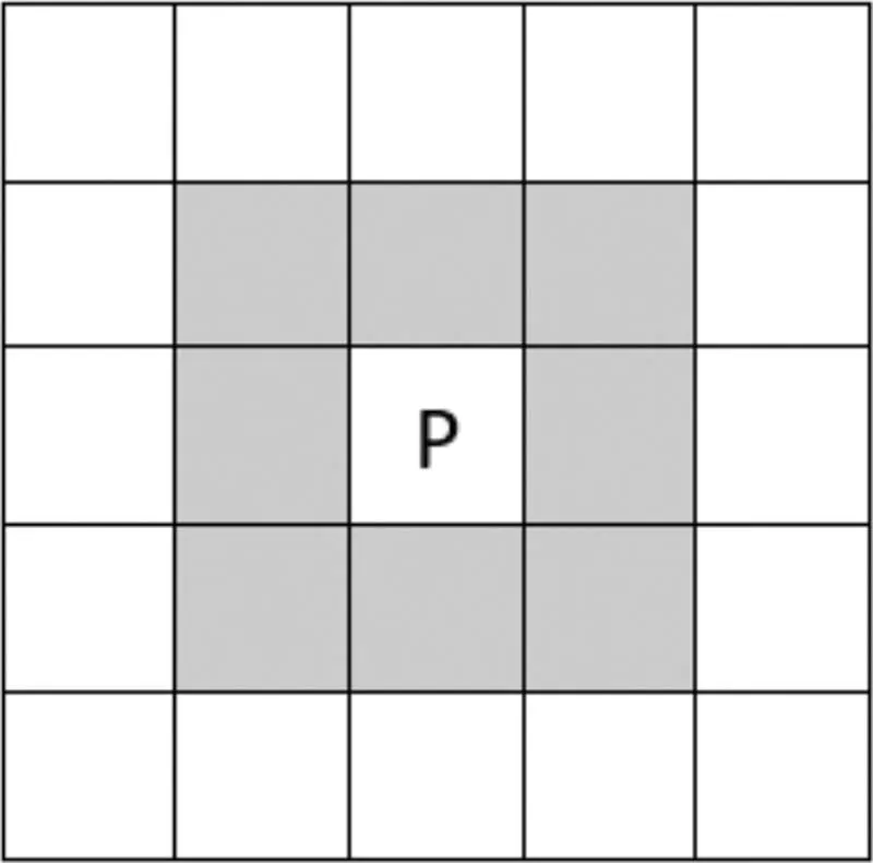
FIGURE 1.1
The grey pixels form the neighborhood of the pixel “P”.

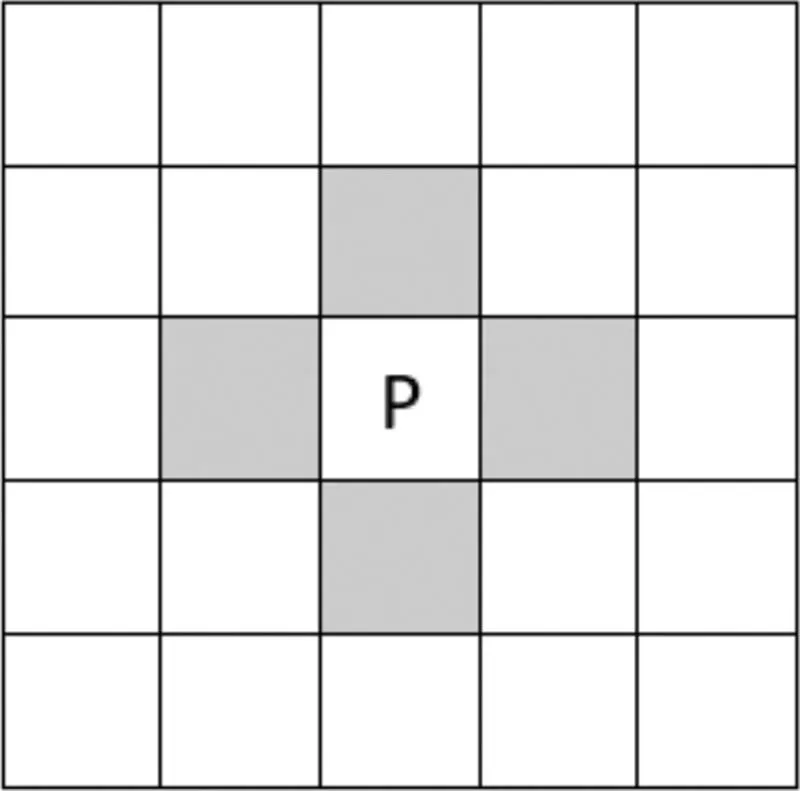
FIGURE 1.2
The grey pixels for the 4-neighbourhood of the pixel “P”.

1.1.2 d-Neighborhood

This neighborhood is composed of those pixels that do not touch, or they touch the corners [4]. That is, the diagonal pixels as shown in Figure 1.3.

1.1.3 8-Neighborhood

This is the union of the 4-neighborhood and the d-neighborhood [5]. It is the maximum probable neighborhood that a pixel can have as shown in Figure 1.4.

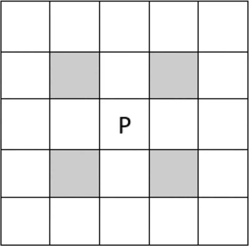
FIGURE 1.3
The diagonal neighborhood of the pixel “P” is shown in color.

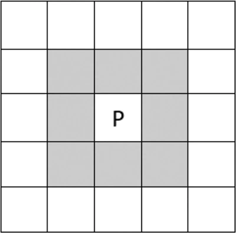
FIGURE 1.4
The 8-neighborhood.

1.1.4 Connectivity

Two pixels are supposed to be “connected” if they belong to the neighborhood of each other as shown in Figure 1.5.

The entire grey pixels are “connected” to “P” or they are 8-connected to “P”. Therefore, only the dark grey ones are 4-connected to “P”, and the light grey ones are d-connected to “P”.

If there are several pixels, they are said to be connected if there is some “chain-of-connection” among any two pixels as shown in Figure 1.6.

Here, let’s say the white pixels are considered the foreground set of pixels or the shape pixels. Then, pixels P₂ and P₃ are connected. There exists a chain of pixels which are connected to each other. However, pixels P₁ and P₂ are not connected. The black pixels (which are not in the foreground set of pixels) block the connectivity.

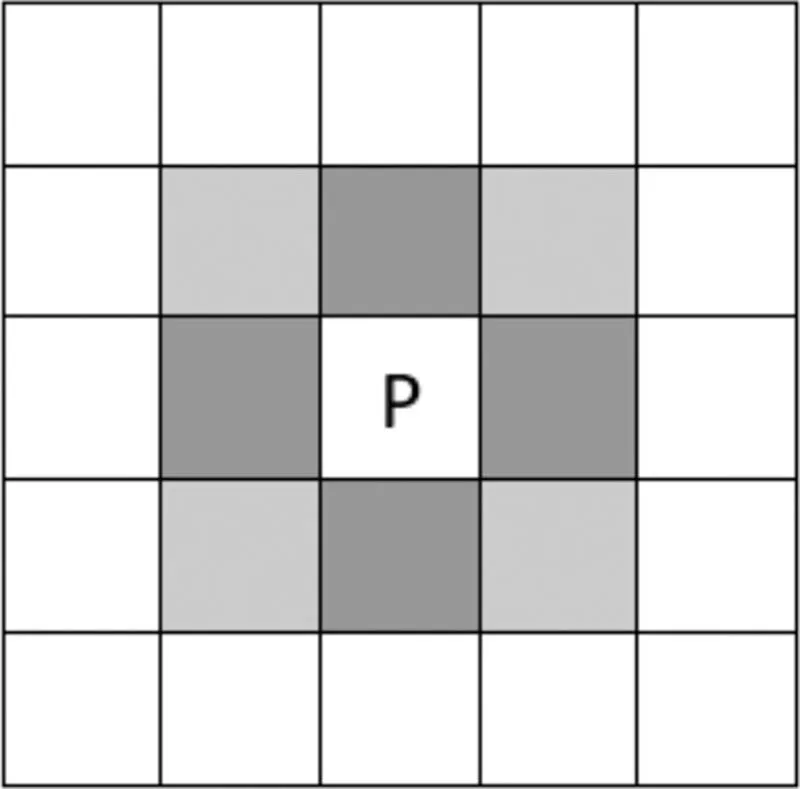
FIGURE 1.5
Connectivity of pixels.

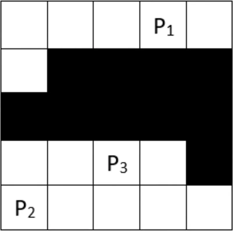
FIGURE 1.6
Multiple connectivity.

1.1.5 Connected Components

Taking the idea of connectivity, the idea of connected components is generated [6]. A graphic that best serves to clarify this idea is shown in Figure 1.7.

Figure 1.8 shows the connected component labeling example.

Each connected region has exactly one value (labeling).

Shapes can be represented in cartesian or polar coordinates. A cartesian coordinate (Figure 1.9a) is the simple x-y coordinate, and in polar coordinates (Figure 1.9b), shape elements are represented as pairs of angle θ and distance r.

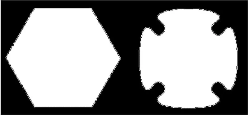
FIGURE 1.7
Connected components.

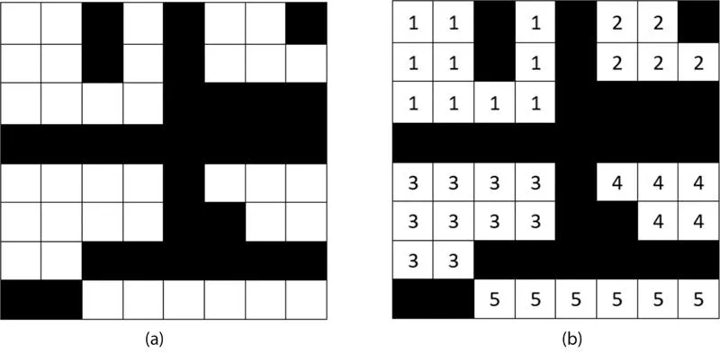
FIGURE 1.8
(a) Original image, (b) connected component labeling.

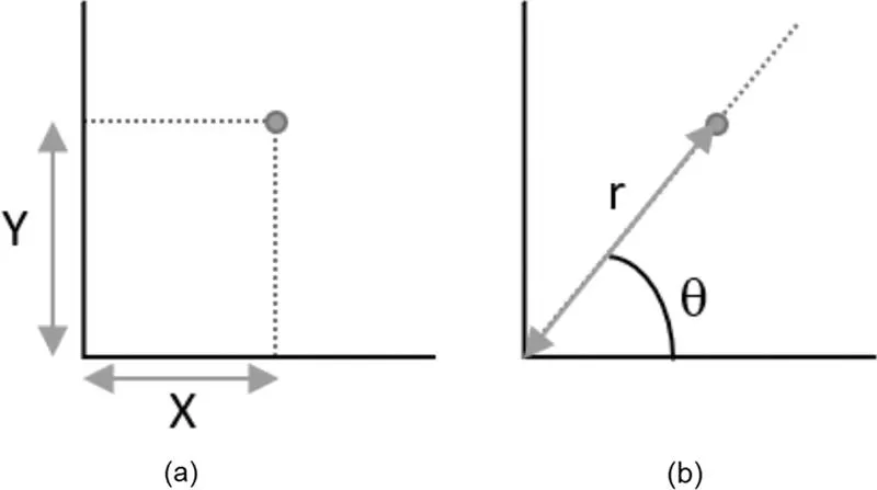
FIGURE 1.9
Coordinate system: (a) cartesian coordinate, and (b) polar coordinate.

1.2 Importance of Shape Features

Shape discrimination or matching refers to approaches for comparing shapes [7]. It is utilized in model-based object recognition where a group of known model objects is equated to an unidentified object spotted in the image. For this purpose, a shape description scheme is utilized to determine the shape descriptor vector for every model shape and unidentified shape in the scene. The unidentified shape is matched to one of the model shapes by equating the shape descriptor vectors utilizing a metric. In Figure 1.10b the grey-scale image of the original image is shown, in Figure 1.10c an overall shape of a leaf is presented, while boundary shape and interior details are illustrated in Figure 1.10d.

The basic idea by simple shape examples is illustrated in Figure 1.11. Shapes in Figure 1.11a–c are rotationally symmetric, and by this feature they can be differentiated from the shapes in Figure 1.11d and e.

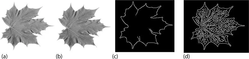
FIGURE 1.10
Shape representation. (a) Original image; (b) Grey-scale image; (c) Overall shape; (d) Boundary shape and interior details.

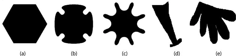
FIGURE 1.11
(a–e) Shape examples.

Assume a shape function S₁ is defined as a “symmetricity” measure. Additionally, since S₁ doesn’t differentiate between the shapes in Figure 1.11a–c, another shape descriptor should be measured. Since the shape in Figure 1.11a is convex, and as the shape in Figure 1.11b is “more convex” than shape in Figure 1.11c, a “convexity” measure (i.e., another shape function) S₂ is considered. S₂ is probable to assign 1 to convex shapes and smaller values for “less convex” shapes (e.g., 0.92 to the shape in Figure 1.11b and 0.75 to the shape in Figure 1.11c). Such a demarcated function would differentiate among the shapes in Figure 1.11d and e, but it is not clear whether it is able to differentiate between shapes in Figure 1.11b and d. It is hard to judge which of them is “more convex”. To overcome such a problem, another descriptor (e.g., shape “linearity”) could be involved. A linearity measure S₃ should allocate a high value to the shape in Figure 1.11...

Table of contents

• Cover
• Half Title
• Title Page
• Copyright Page
• Table of Contents
• Preface
• Authors
• 1. Introduction to Shape Feature
• 2. One-Dimensional Function Shape Features
• 3. Geometric Shape Features
• 4. Polygonal Approximation Shape Features
• 5. Spatial Interrelation Shape Features
• 6. Moment Shape Feature
• 7. Scale-Space Shape Features
• 8. Shape Transform Domain Shape Feature
• 9. Applications of Shape Features
• Index