Linear Programming and Algorithms for Communication Networks

A Practical Guide to Network Design, Control, and Management

Eiji Oki

• Publisher: CRC Press
• Year: 2012
• Print ISBN: 9781466552630
• eBook ISBN: 9781466578609
• Edition: 1
• Topic: Computer Science
• Subtopic: Information Technology
• Index: Computer Science

Explaining how to apply to mathematical programming to network design and control, Linear Programming and Algorithms for Communication Networks: A Practical Guide to Network Design, Control, and Management fills the gap between mathematical programming theory and its implementation in communication networks. From the basics all the way through to m

Chapter 1

Optimization problems for communications networks

Communication networks consist of nodes and links. Figure 1.1 shows an example of a network. This network consists of six nodes, node 1 to node 6. An arrow between two nodes is a connection, called a link, of those nodes. The traffic has a direction from the tail to the head of the arrow. For example, the arrow from node 1 to node 2 means that node 1 and node 2 are connected and the traffic flows from node 1 to node 2. The network in which each link has a direction, represented by a corresponding arrow, as shown in Figure 1.1, is called a directed graph. A number on each link indicates its link cost. In the case that the connection is represented by just a line, instead of an arrow, the traffic can flow in both directions on the link. A network with links through which the traffic flows in both directions is called a undirected graph.

This chapter introduces typical examples of the problems posed by communication networks, starting with the shortest path problem.

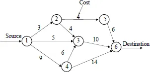
Figure 1.1: Network model with link costs.

1.1 Shortest path problem

Consider that node 1 wants transmit traffic to node 6, as shown in Figure 1.1. We need to find the path with the minimum cost to transmit the traffic. Nodes 1 and 6 are called source and destination nodes, respectively. The path with the minimum cost from the source node to the destination node is called the shortest path. The shortest path is determined by considering the link costs in the network. This problem is called the shortest path problem. The problem is solved and the solution is obtained, as shown in Figure 1.2. The shortest path from node 1 to node 6 is 1 → 2 → 5 → 6, and the path cost, which is the sum of costs of the links on the path, is 3 + 4 + 6= 13.

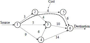
Figure 1.2: Shortest path from node 1 to node 6.

1.2 Max flow problem

Figure 1.3 shows a network that considers the capacity of each link. The number on each link represents the link capacity; that is the maximum traffic that can be transmitted through the link. Traffic volume, v, is injected from node 1. How much maximum traffic can we send from node 1 to node 6? Which route should the traffic be transmitted on? This problem is called the max flow problem. Figure 1.4 shows the solution of this problem. The maximum traffic volume from node 1 to node 6 is v = 195 and consists of five paths with their corresponding traffic volumes of v₁ to v₅. v₁ = 15 is sent on the first path, 1 → 2 → 5 → 6. v₂ = 10 is sent on the second path, 1 → 2 → 3 → 6. v₃ = 100 is sent on the third path, 1 → 3 → 6. v₄ = 60 is sent on the fourth path, 1 → 4 → 3 → 6. v₅ = 10 is sent on the fifth path, 1 → 4 → 6. The total traffic v is v₁ + v₂ + v₃ + v₄ + v₅ = 15 + 10+100 + 60+10 = 195. The traffic that flows on each link does not exceed the link capacity. For example, the traffic on link 1 → 2 is v₁ + v2 = 15 + 10 = 25, which does not exceed 25 (25 is the capacity of link 1 → 2). The traffic on link 3 → 6 is v₂ + v₃ + v₄ = 10 + 100 + 60 = 170 does not exceed 200 (200 is the capacity of link 1 → 2).

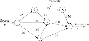
Figure 1.3: Network model with link capacities.

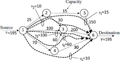
Figure 1.4: Max flow routing from node 1 to node 6.

1.3 Minimum-cost flow problem

Figure 1.5 shows a network that considers the cost and capacity of each link. The numbers on each link represents the link cost and the link capacity. The traffic flow cannot exceed the link capacity. The traffic volume that is required to be transmitted from a source node, node 1, to a destination node, node 6, is set to v = 180. How can we send the required traffic volume from node 1 to node 6 at the minimum cost? This problem is called the minimum-cost flow problem. In the minimum-cost flow, the required cost for each link is defined as the cost of the link × the traffic volume that flows on the link. We minimize the sum of costs on the path(s) to send the traffic from node 1 to node 6.

Figure 1.6 shows the solution of the minimum-cost flow problem. The traffic with the volume of v is divided into five paths, from v₁ to v₅. v₁ = 15 is sent on the first path, 1 → 2 → 5 → 6. v₂ = 10 is sent on the second path, 1 → 2 → 3 → 6. v₃ = 100 is sent on the third path, 1 → 3 → 6. v₄ = 25 is sent on the fourth path, 1 → 4 → 3 → 6. v₅ = 30 is sent on the fifth path, 1 → 4 → 6. The total traffic volume is v = v₁ + v₂ + v₃ + v₄ + v₅ = 15 + 10 + 100 + 25 + 30 = 180. The total cost is 3180. There is no traffic flow that exceeds the capacity of the link on which it flows.

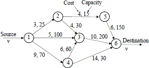
Figure 1.5: Network with link costs and capacities.

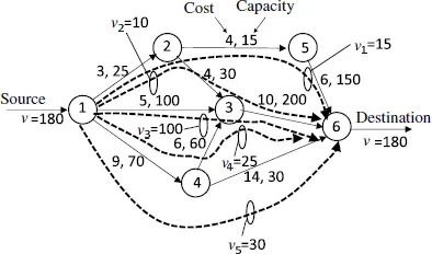
Figure 1.6: Minimum-cost flow from node 1 to node 6.

Chapter 2

Basics of linear programming

An optimization problem is a problem that aims to find the best solution from all feasible solutions. The best solution can be the minimum or maximum solution. An example of the former is finding the route from point A to point B that takes the shortest time. An example of the latter is determining how a production factory can maximize its profit using limited materials. Both problems are optimization problems. An optimization problem can be solved by mathematical programming, a technique that expresses and solves problems as mathematic models.

This chapter explains linear programming, which is a special case of mathematical programming.

2.1 Optimization problem

A businessman must travel from city A to city B on a business trip. He has two choices as to the means of transportation: airplane or train. How can he travel with the minimum cost given the following conditions?

• Condition 1: The price for a one-way ticke...

Table of contents

• Cover
• Title Page
• Copyright
• Contents
• Preface
• 1 Optimization problems for communications networks
• 2 Basics of linear programming
• 3 GLPK (GNU Linear Programming Kit)
• 4 Basic problems for communication networks
• 5 Disjoint path routing
• 6 Optical wavelength-routed network
• 7 Routing and traffic-demand model
• 8 IP routing
• 9 Mathematical puzzles
• A Derivation of Eqs. (7.6a)–(7.6c) for hose model
• B Derivation of Eqs. (7.12a)–(7.12c) for HSDT model
• C Derivation of Eqs. (7.16a)–(7.16d) for HLT model
• Answers to Exercises
• Index