OSPF and IS-IS

From Link State Routing Principles to Technologies

Rui Valadas

• Publisher: CRC Press
• Year: 2019
• Print ISBN: 9781138504554
• eBook ISBN: 9780429648489
• Edition: 1
• Topic: Computer Science
• Subtopic: Computer Networking
• Index: Computer Science

This book describes and compares both the IPv4 and IPv6 versions of OSPF and IS-IS. It explains OSPF and IS-IS by grounding the analysis on the principles of Link State Routing (LSR). It deliberately separates principles from technologies. Understanding the principles behind the technologies makes the learning process easier and more solid. Moreover, it helps uncovering the dissimilarities and commonalities of OSPF and IS-IS and exposing their stronger and weaker features. The chapters on principles explain the features of LSR protocols and discuss the alternative design options, independently of technologies. The chapters on technologies provide a comprehensive description of OSPF and IS-IS with enough detail for professionals that need to work with these technologies. The final part of the book describes and discusses a large set of experiments with Cisco routers designed to illustrate the various features of OSPF and IS-IS. In particular, the experiments related to the synchronization mechanisms are not usually found in the literature.

Part IV

Case studies

8

Tools and Configurations

Experimenting is an important step in acquiring effective skills in computer networking. You cannot become a computer networking specialist just by reading books! Well, this part of the book proposes and discusses a large number of experiments that illustrate the main features of OSPF and IS-IS. The experiments were designed so that they can be easily reproduced by the reader (and some of them are really fun!). They require IP routers implementing single-area and hierarchical OSPF and IS-IS for both IPv4 and IPv6 networks, and a protocol analyzer. However, they can be performed in an emulated environment, i.e. using only the operating system of routers and not the real equipment. In our experiments we have used GNS3 as the network emulator, a Cisco IOS image as the router operating system, and Wireshark as the protocol analyzer.

Structure of this part of the book This chapter presents the main features of GNS3, Cisco IOS, and Wireshark, and explains the basic router configurations. The next chapters discuss several types of experiments. Chapter 9 addresses the structure of the forwarding tables, the route selection process, and the LSDB structure of single-area networks. Chapter 10 discusses the synchronization mechanisms. Finally, Chapter 11 addresses the extensions required to support hierarchical networks.

Two words of caution There are no perfect specifications and no perfect implementations of LSR protocols, nor are the tools used to emulate and analyze them perfect (as anything in our lives…). Thus, when running experiments with LSR protocols, you may be faced with unexpected behavior due to unclear specifications, implementation bugs, undocumented vendor specific features, intrinsic hardware and software limitations, and so on. However, most of the time the unexpected behavior arises because you failed to understand that specific bit of the protocol… So, be prepared for the surprises!

LSR protocols are asynchronous protocols. One feature of this type of protocol is that the sequence of events leading to a given outcome may vary. For example, the sequence of LS UPDATE packets transmitted on a shared link in reaction to some router failure depends (i) on the relative timing of the failure detection by the neighbors of the failed router, and (ii) on the load of the routers and links in the various routes between the neighbors and the shared link. The beauty of asynchronous protocols—if they are correct—is that the outcome is always the same irrespective of the sequence of events. Thus, always be prepared for a different sequence of events when you try to reproduce the experiments of this part of the book.

What is a converged network? We will refer many times to converged networks. A converged network is a network in a stable state. In the context of routing protocols, this means that the routing information used to build the forwarding tables is not changing and is consistent across all routers. Following an event such as a router failure or a cold start, there is usually a transient period when the network is adapting to the new conditions and the routing information changes; however, if the protocol is correct, the routing information becomes stable after a while. Thus, network convergence is always the endpoint of LSR experiments that disturb the network stability.

One way to determine if a network has converged in LSR experiments is to observe the control packets transmitted by the routers, e.g. using Wireshark. The conditions differ slightly in OSPF and IS-IS. In OSPF, a converged network is a network where only HELLO packets with correct information are exchanged between routers. The information transmitted by an HELLO packet is correct if it lists all neighbors of the sending router and, on shared links, if it also lists the correct DR and BDR. The IS-IS conditions are the same, except on shared links, where, besides the HELLO packets transmitted by all routers, the DIS also transmits periodic CSNPs. In this case, network convergence is achieved when the routers transmit only correct HELLO packets, and the DISes, besides correct HELLO packets, also transmit CSNPs advertising a fully updated LSDB summary.

8.1 Getting used to GNS3

GNS3 is a network emulator that allows testing network configurations using the actual operating system of networking equipment (e.g. Cisco IOS or Juniper JUNOS) and using Wireshark for packet analysis. In our experiments we have used version 2.1.3 of GNS3.

To perform experiments with Cisco devices you must install first a Cisco IOS image. Other elements such as the links, the Ethernet switches, and the PCs are provided by GNS3.

Central pane Figure 8.1 shows the main window of GNS3. The central pane displays the network you have configured. In this case, the network has five routers (R1 to R5) connected through Fast Ethernet links, except the connection between R4 and R5, which is a serial link. Moreover, router R5 is connected to an Ethernet switch. The interfaces are labeled with their names.

Left pane The network devices can be drag-and-dropped from the left pane, where they are organized in categories. For example, in the first button (Browse Routers) you find the routers, in the second one (Browse Switches) the switches, and in the last one (Add a link) the links. These are the network elements that you need for almost all experiments of this book.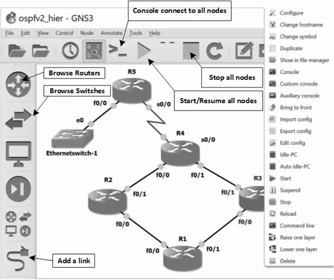

FIGURE 8.1: GNS3 main window.

Upper pane The upper pane includes buttons for the main actions performed on a network. For example, to start all devices at the same time click Start/Resume all nodes, and to stop them all click Stop all nodes. The button Console connect to all nodes is also very useful and opens the consoles of all devices at the same time.

Performing actions on individual devices There are many actions that you can perform on individual devices. For that, you must right click the device. Figure 8.1 shows the window that opens when right clicking router R3. You can, for example, Start, Stop, or Reload just this router, you can open its console (Console button), configure the router (Configure button), or edit its startup-config file (Edit config button). In addition, to run a Wireshark capture at a link, right click on the link and select Start capture.

These are just the main features of GNS3; try to explore other features on your own. Have fun!

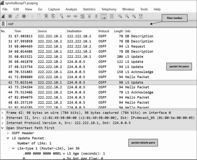
FIGURE 8.2: Wireshark main window.

8.2 Getting used to Wireshark

Wireshark is a protocol analysis tool. It can capture all packets that cross a network interface (in both directions) and decode their complete contents, e.g. it identifies the protocols of the various layers and the source and destination addresses. It is a very useful tool for computer networking specialists. Moreover, Wireshark is fully integrated with GNS3. When emulating a network using GNS3, several Wireshark captures can be run simultaneously, to observe different points of the network. We could not have a better environment to study computer networks! Moreover, Wireshark is easy to install and to work with. In our experiments, we have used version 2.4.4 of Wireshark.

Figure 8.2 shows the main window of Wireshark. In this case, the window shows information on the packets exchanged during an initial LSDB synchronization in OSPF. We highlight three main areas: (i) the filter toolbar, (ii) the packet list pane, and (iii) the packet details pane.

Filter toolbar A filter lets you choose what you want to see. In Wireshark, the filters are specified in the filter toolbar, and there are many predefined filters. For example, the ospf keyword, shown in Figure 8.2, lets us see only OSPF packets. In our experiments, we will use ospf or isis filters. Wireshark allows us to be more specific regarding a protocol. For example, to see only OSPF HELLO packets you can use the ospf.hello filter. Packet list pane Immediately below the filter toolbar, you find the packet list pane. This pane has one line per observed packet and displays the most important information regarding each packet. It has seven columns: (i) No. is the packet number, (ii) Time is the capture time, (iii) Source is the source address, (iv) Destination is the destination address, (v) Protocol is the highest-layer protocol decoded by Wireshark, (vi) Length is the packet length, and (vii) Info includes additional information, such as the packet type.

The packet number and the packet capture time are relative to the first observed packet. The first observed packet is given a number of 1 and a capture time of 0. The source and destination addresses are the IP addresses, unless the packet has no IP layer (which is the case of the IS-IS packets); in this case, the source and destination MAC addresses (if they exist) are displayed.

Packet details pane Below the packet list pane, you find the packet details pane. This pane shows all fields of the packet selected in packet list pane. In the figure, the packet selected is packet 42 (an LS UPDATE packet) and the packet details pane shows its Ethernet and IPv4 headers (not expanded), and shows that the OSPF packet contains a Router-LSA with an LS Age of 1 second (most of the contents is not shown due to lack of space).

How Wireshark captures will be shown in this book In this book we will show the results of many Wireshark captures. However, we will not present them as in Figure 8.2, i.e. as Wireshark snapshots, because we want to save space and add important information not displayed in the packet list ...

Table of contents

• Cover
• Half Title
• Title Page
• Copyright Page
• Dedication
• Table of Contents
• Preface
• I Introduction
• II Principles
• III Technologies
• IV Case studies
• Glossary
• References
• Index