R For College Mathematics and Statistics

Thomas Pfaff

• Publisher: Chapman and Hall/CRC
• Year: 2019
• Print ISBN: 9781032475684
• eBook ISBN: 9781000006971
• Topic: Economía
• Subtopic: Estadísticas para los negocios y la economía

R for College Mathematics and Statistics encourages the use of R in mathematics and statistics courses. Instructors are no longer limited to ``nice'' functions in calculus classes. They can require reports and homework with graphs. They can do simulations and experiments. R can be useful for student projects, for creating graphics for teaching, as well as for scholarly work. This book presents ways R, which is freely available, can enhance the teaching of mathematics and statistics.

R has the potential to help students learn mathematics due to the need for precision, understanding of symbols and functions, and the logical nature of code. Moreover, the text provides students the opportunity for experimenting with concepts in any mathematics course.

Features:

• Does not require previous experience with R
• Promotes the use of R in typical mathematics and statistics course work
• Organized by mathematics topics
• Utilizes an example-based approach
• Chapters are largely independent of each other

1

Getting Started

If you do not have R on your desktop then download it now from https://www.r-project.org/. When you click on download R, you will first be asked to choose a CRAN mirror, a location to download the software from, and then will be to a page to choose between Windows, Mac, or Linux. Following the Download R for Windows link will take you to the page for Windows that has a download R for the first time link. After that link you will be directed to a page with a download link at the top. Following the Download R for (Mac) OS X link takes you to a download R for Mac OS X page. Click on the first link on the left under the Latest release header. Linux users can follow the Download R for Linux link. In all cases you can search for videos if you are having difficulties loading R.

When you open R you will see the R Console box with > prompt. Take a few moments and play with R as a calculator with * as multiplication and for exponents. For example we calculate 2^{^}6*3*643.

R Code

> 2^6*3*643

[1] 123456

Throughout this text these boxes will represent the R code and its output. Now that you are comfortable using the R console we want to stop using it as our primary input method as scripts are preferred. Open up a new script (document for Macs) by going to File -> New script. A new window opens with the name Untitled – R Editor. Save this file to a location of your choosing and name it FirstScript and note that it is a .R filetype. The R Editor allows you to type your commands and edit them before you run them in the R console. The file can also be saved for future reference and reuse.

Working in the R Editor

• Text following # will be ignored by R. This is how you add comments to your commands so that you can easily read them later.

• Ctrl + R (Command Return with a Mac) will send the current line in the editor to the console. Similarly, any highlighted commands in the editor will be sent to the console when you press Ctrl + R.

• A + sign in the R console means that R is expecting something more. For example you might be missing a parenthesis or bracket. To get out and back to the > prompt use the Esc key.

• Recognize that your toolbar and submenu options depend on which window, console or editor, is selected.

Here are two quick examples to get started, but first a few conventions of this book. R code is taken from the console and so lines of code are preceded by >. If a line does not have a > then the line above was broken and started a new line to fit the page. It is meant to be part of the single line started above and preceded by >. A line that starts with a + is, in fact, a separate line of code, but is part of a larger collection of code. The code in this book uses color, but to see the color you will need to run the code as this book is in black and white.

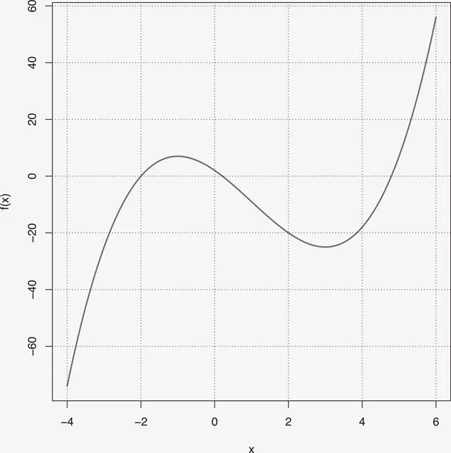
The first example, graphs the function f (x) = x³ – 3x² – 9x + 2 on the interval [−4, 6]. To do this, we first define the function. The syntax sets f equal to function(x), a function with variable x, with the expression defined enclosed in braces. Note that * is necessary to represent multiplication. Entering 9x will generate an error as it must be 9*x. The curve function here has five input elements separated by a comma. The first is the function to be graphed. The next two define the x-axis interval for the graph. The first three entries are not optional and must be in this order. The next two elements are optional and can be in any order. We set lwd=2 for the line width and col to red, in quotes, for the color of the graph. A grid is added with grid. The first two elements, NULL, set the grid lines to the tick marks given by the graph created with curve. There are other options here that can be used. The last entry sets the color of the grid lines, with a default of gray. To add another function to the graph, curve can be used again, but the option add=TRUE must be included. To learn more about curve and grid run ?curve or ?grid, which will open a webpage with details about the functions. In general, a question mark followed by a command will open an R documentation page with details about the command.

R Code

> f=function(x){x^3-3*x^2-9*x+2}

> curve(f,-4,6,lwd=2,col="red")

> grid(NULL,NULL,col="black")

The next example begins by generating a random data set of size 150 from a random normal distribution with mean 0 and standard deviation 1. The data returned by rnorm is set to the variable example. At this point example is a vector of length 150. We use summary to return the five number summary plus the mean of the data set example. Note, that the data set is randomly generated so results will differ. Use set.seed(42) to get the same results. We can use sd(example) for the standard deviation and boxplot(data) to create a boxplot of the data.

R Code

> example=rnorm(150,0,1)

> summary(example)

Min. 1st Qu. Median Mean 3rd Qu. Max.

−2.99309 −0.61249 −0.04096 −0.02874 0.64116 2.70189

For an example of a t-test, we test the data example with an alternative of μ < 0. The function t.test() is used. The first entry is the data and is not optional. The other three inputs set the value of μ₀ to 0, the alternative hypothesis to less than, and the confidence level to 0.90. The default μ₀ is 0 so this isn’t necessary here. The default alternative is two-sided and the options for alternative are two.sided, less, and greater and must be in quotes. The default confidence level is 0.95. To learn more about these functions run?t.test or ?boxplot, for example.

R Code

> t.test(example,mu=0,alternative="less", conf.level=0.90)

One Sample t-test

data: example

t = -0.35007, df = 149, p-value = 0.3634

alternative hypothesis: true mean is less than 0

90 percent confidence interval:

-Inf 0.07694166

sample estimates:

mean of x

-0.02874049

At this point, you should feel free to explore the chapters. The next section is specifically for importing data into R that you may not need at the moment. Depending on your interests, two good chapters to turn to next are Chapter 2, Functions and Their Graphs or one of the basic statistics chapters, Chapters 11, 12, or 13. One last tip: Some chapters use a package. A package can be thought of as an add-on to R that does something more than the base distribution. There are over 10,000 packages for R. To use a package, it must first be downloaded, which only has to be done once. To download a package, make sure the console window is highlighted and use the package menu along the top. You will first need to select as CRAN location, as is done when loading R, and then select the package. Search load package in R if there are any difficulties. When you want to use a particular package run library(name), which you will see in this book anytime a package is used.

1.1 Importing Data into R

One of the strengths of R is statistical computing, but entering large data sets directly into R is not a common practice. Typically, for colleges mathematics and statistics courses, your data will come from a spreadsheet and you will want to import that data into R. The example below assumes that a csv file has been created, likely from Excel, from the Arctic Sea Ice data from Appendix B.

Importing a csv File

• Make sure your csv file is free of commas and apostrophes within cells, has only one tab, and you have deleted unnecessary cells. Also, your first cell cannot be named ID.

• With the Console window selected go to File -> Change dir… and select the folder that contains the csv file. In a Mac, Change Dir is under Misc.

• Enter the command DataName=read.table(“File Name.csv”, header=TRUE, sep=“,”). Here DataName gives the data a name within the R environment. Choose a meaningful name. Note header=TRUE tells R that you have column nam...

Table of contents

• Cover
• Half Title
• Title Page
• Copyright Page
• Dedication
• Table of Contents
• Preface
• Acknowledgments
• 1 Getting Started
• 2 Functions and Their Graphs
• 3 Graphing
• 4 Polynomials
• 5 Sequences, Series, and Limits
• 6 Calculating Derivatives
• 7 Riemann Sums and Integration
• 8 Planes, Surfaces, Rotations, and Solids
• 9 Curve Fitting
• 10 Simulation
• 11 The Central Limit Theorem and Z-test
• 12 The T-Test
• 13 Testing Proportions
• 14 Linear Regression
• 15 Nonparametric Statistical Tests
• 16 Miscellaneous Statistical Tests
• 17 Matrices
• 18 Differential Equations
• 19 Some Discrete Mathematics
• A Loops, Vectors, and Apply
• B Arctic Sea Ice Data
• Bibliography
• Index