Digital Photogrammetry

Yves Egels, Michel Kasser

• Publisher: CRC Press
• Year: 2001
• eBook ISBN: 9781135730390
• Edition: 1
• Topic: Technology & Engineering
• Subtopic: Civil Engineering
• Index: Technology & Engineering

Photogrammetry is the use of photography for surveying primarily and is used for the production of maps from aerial photographs. Along with remote sensing, it represents the primary means of generating data for Geographic Information Systems (GIS). Digital Photogrammetry is a unique book in that it examines the digital aspect of photogrammetry and delves into topics like acquisition of data, workstations, digital tools, Orthophotography, and more. This book is particularly useful as a text for graduate students in geomantics, but is also suitable for people with a good basic scientific knowledge who need to understand photogrammetry, and who wish to use the book as a reference.

1 Image acquisition. Physical aspects. Instruments

INTRODUCTION

We may define photogrammetry as ‘any measuring technique allowing the modelling of a 3D space using 2D images’. Of course, this is perfectly suitable for the case where one uses photographic pictures, but this is still the case when any other type of 2D acquisition device is used, for example a radar, or a scanning device: the photogrammetric process is basically independent of the image type. For that reason, we will present in this chapter the general physical aspects of the data acquisition in digital photogrammetry. It starts with §1.1, a presentation of the geometric aspects of photogrammetry, which is a classic problem but whose presentation is slightly different from books dealing with traditional photogrammetry. In §1.1 there are also some considerations about atmospheric refraction, the distortion due to the optics, and a few rules of thumb in planning aerial missions where digital images are used. In §1.2, we present some radiometric impacts of the atmosphere and of the optics on the image, which helps to understand the very physical nature of the aerial images. And in §1.3, these few lines about colorimetry are necessary to understand why the digital tools for managing black and white panchromatic images need not be the same as the tools for managing colour images. Then we will present the instruments used to obtain the images, digital of course. In §1.4 we will consider the geometric constraints on optical image acquisitions (aerial, and satellite as well). From §1.5 to §1.8, the main digital acquisition devices will be presented, CCD cameras (§1.5), radars (§1.6), airborne laser scanners (§1.7), and photographic image scanners (§1.8). And we will close this chapter with an analysis of the key problem of the size of the pixel, and the signal-to-noise ratio in the image.

1.1 MATHEMATICAL MODEL OF THE GEOMETRY OF THE AERIAL IMAGE

Yves Egels

The geometry of images is the basis of all photogrammetric processes, analogical, analytic or digital. Of course, the detailed geometry of an image essentially depends on the physical features of the sensor used. In analytic photogrammetry (the only difference with digital photogrammetry is the digital nature of the image) the use of this technology of image acquisition requires therefore a complete survey of its geometric features, and of the mathematical tools expressing the relation between the coordinates on the image and those of ground points (and, if the software is correct, this will be the only thing to do).

We shall explain here, just as an example, the case of the traditional conical photography (the image being silver halide or digital), that is still today the most used and that will be able to be a guide for the analysis of a different sensor. The leading principle, here as well as in any other geometrical situation, is to approach the quite complex real geometry by a simple mathematical formula (here the perspective) and to consider the differences between the physical reality and this formula as corrections (‘corrections of systematic errors’) presented independently. The imaging devices whose geometry is different are presented later in this chapter (§§1.4 to 1.7).

1.1.1 Mathematical perspective of a point of the space

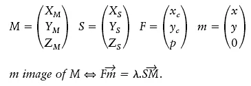
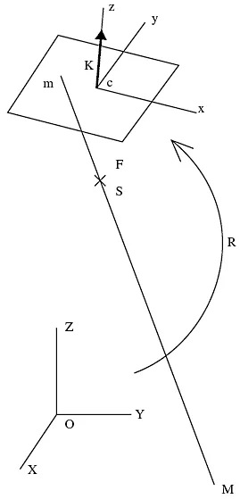
The perspective of a point M of the space, of centre S, on the plane P is the intersection m of the line SM with the plane P. Coordinates of M will be expressed in the reference system (O, X, Y, Z), and the ones of m in the reference system of the image (c, x, y, z). The rotation matrix R corresponds to the change of system (O, X, Y, Z) → (c, x, y, z). One will note F the coordinates of the summit S in the reference of the image.

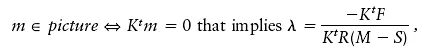
If one calls K the vector unit orthogonal to the plane of the image one can write:

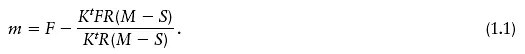
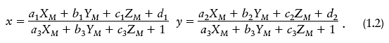
from where the basic equation of the photogrammetry, so-called collinearity equation:

s

Figure 1.1.1 Systems of coordinates for the photogrammetry.

This equation can be developed and reordered according to coordinates of M, under the so-called ‘11 parameters equation’, which appears simpler to use, but should be handled with great care:

1.1.2 Some mathematical tools

1.1.2.1 Representation of the rotation matrixes, exponential and axiator

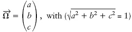
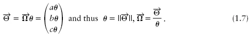
In computations of analytic photogrammetry, the rotation matrixes appear quite often. On a vector space of n dimensions, they depend on n(n – 1)/2 parameters, but do not form a vector sub-space. There is therefore no linear formula between a rotation matrix and its ‘components’. It is, however, vital to be able to express such a matrix judiciously according to the chosen parameters. In the case of R³, it is usual to analyse the rotation as the composition of three rotations around the three axes of coordinates (angles w, ϕ and κ, familiar to photogrammetrists). But the resulting formulas are laborious enough and lack symmetry, which obliges us to perform unnecessary developments of formulas. One will be able to define a rotation of the following manner physically: rotation of an angle θ around a unitary vector

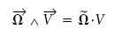
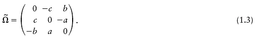
We will call here the axiator of a vector the matrix equivalent to a vectorial product:

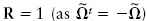
one will check that

It is easy to control that the previous rotation can be written:

. Indeed,

therefore, since

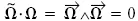
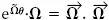
(a well-known property of the vectorial product)

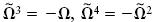
is the rotation axis, only invariant. One will check that

, etc.; on the other hand,

Therefore this matrix is certainly an orthogonal matrix, which is a rotation matrix as det

. One will also verify that the rotation angle is equal to θ, for example by computing the scalar product of a normal vector to Ω with its transform.

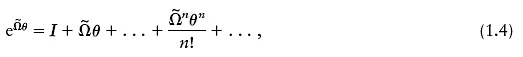
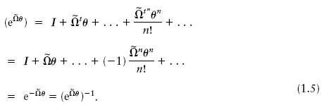
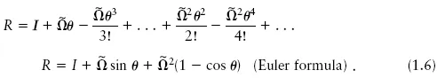
One sees therefore, while regrouping the even terms and the odd terms of the procedure:

This formula will permit a very comfortable calculation of rotations. Indeed one can choose, as parameters of the rotation, the three values aθ, bθ and cθ. One can then write:

If one expresses sin θ and cos θ using tan θ/2 with the help of the classic trigonometric formulas, it becomes:

1.1.2.2 Differential of a rotation matrix

Expressed under this exponential shape, it is possible to differentiate the rotation matrixes. One may determine:

In this expression, the differential makes the parameters of the rotation appear under matrix shape, which is not very practical. Applied to a vector, it can be written (using the anticommutativity of the vectorial product):

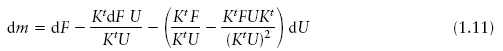
1.1.2.3 Differential relation binding m to the parameters of the perspective

The previous equation is not linear, and to solve systems corresponding to analytical photogrammetry (orientation of images, aerotriangulation), it is necessary to linearize them. Variables that will be taken into account are F, M, S and R.

If one puts A = M – S and U = RA

On the other hand, K^tF being a scalar, K^tFU = UK^tF and K^tdF U = UK^t dF.

One then gets:

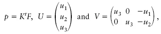
If one writes

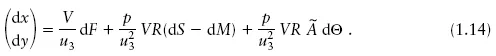
one gets after manipulation:

Under this matrix shape, the computer implementation of this equation requires only a few code lines.

1.1.3 True geometry of images

In physical reality, the geometry of images only reproduces in an approximate way the mathematical perspective whose formulas have just been established. If one follows the light ray from its starting point on the ground until the formation of the image on the sensor, one will find a certain number of differences between the perspective model and the reality. It is difficult to be comprehensive in this area, and one will mention here only the main reasons for distortion whose consequences are appreciable in the photogrammetric process.

1.1.3.1 Correction of Earth curvature

The first reason for which photogrammetrists use the so-called correction of Earth curvature in photogrammetry is that the space in which cartographers operate is not the Euclidian space in which the collinearity equation is set up. It is indeed in a cartographic system, in which the planimetry is measured in a plane representation (often conform) of the ellipsoid, and the altimetry in a system of altitudes.

The best solution for dealing with this is to make rigorous transformations from cartographic to tridimensional frames (it is usually more convenient to choose a local tangent tridimensional reference, if it is necessary just to write relations of planimetric or altimetric conversion in a simple way). This solution, if better in theory, is, however, a little difficult to put into an industrial operation, because it requires having a database of geodesic systems, of projection algorithms (sometimes bizarre) used in the client countries, and arranging a model of the zero level surface (close to the geoid) of the altimetric system concerned.

An approximate solution to this problem can nevertheless be found, that is – experience proves it – of comparable precision with the precision of this measurement technique. It relies on the fact that all conform projections are locally equivalent, with only a changing scale factor. One can attempt to replace the real projection, in which is expressed the coordinates of the ground, by a unique conform projection therefore (and why not try for simplicity!), for example a stereographic oblique projection of the mean curvature sphere on the tangent plane to the centre of the work.

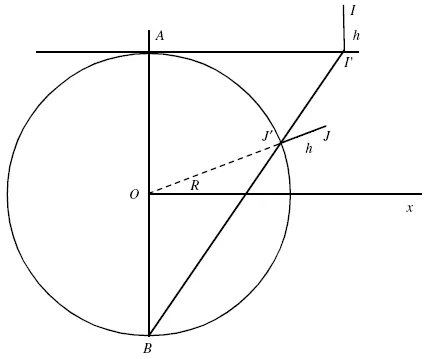
The mathematical formulation then becomes as shown in Figure 1.1.2 (the figure is made in the diametrical plane of the sphere containing the centre of the work A and the point I to transform).

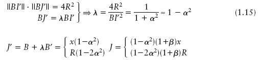
I is the point to transform (cartographic), J the result (tridimensional), I′ the projection of I on the plane and J′ the projection of J on the terrestrial sphere of R radius. I′ and J′ are the inverse of each other in an inversion of B pole and coefficient 4R².

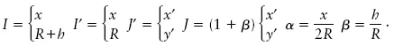
Let us put:

The calculation of the inversion gives:

Figure 1.1.2 Figure made in the diametrical plane of the sphere containing the centre of the work A and the point I to transform.

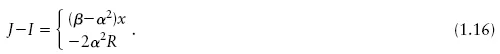
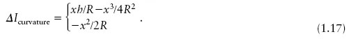
One can consider that J – I corresponds to a correction to bring us to the coordinates of I:

In the current conditions, the term of altimetric correction is by far the most meaningful. But for aerotriangulations of large extent, planimetric corrections can become important, and must be considered. If the aero-triangulation relies on measures of an airborne GPS (global positioning system), it is necessary not to forget also to do this correction on coordinates of tops, that also have to be corrected for the geoid–ellipsoid discrepancy.

1.1.3.2 Atmospheric refraction

Before penetrating the photographic camera, the luminous rays cross the atmosphere, whose density, and therefore refractive index, decreases with the altitude (see Table 1.1.3).

Table 1.1.3 Atmospheric co-index of refraction–variations with the altitude

This variation of the index provokes a curvature of the luminous rays (oriented downwards) whose amplitude depends on atmospheric conditions (pressure and temperature at the time of the image acquisition), that are not uniform in the field of the camera, and are generally unknown.

Nevertheless, this deviation is small with regard to the precision of photogrammetric measurements (with the exception of very small scales). It will thus be acceptable to correct the refraction using a standard reference atmosphere: in order to evaluate the influence of the refraction, it will be necessary to use a model providing the refraction index at various altitudes.

Numerous formulas exist allowing an evaluation of the variation of the air density according to altitude. No one is certainly better that any other, because of the strong turbulence of low atmospheric layers. In the tropospheric domain (these formulas would not be valid if the sensor is situated in the stratosphere), one will be able to use, for example, the formula published by the OACI (Organisation de l’Aviation Civile Internationale):

where

a = –2.560.10^-8, b = 7.5.10^-13, n₀ = 1.000278 h in metres,

or this one, whose integration is simpler:

where

a = 278.10^-6, b = 105.10^-6.

The rays appear to come then from a point situated in the extension of the tangent to the ray at the entrance into the optics, thus introducing a displacement of the image.

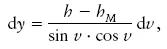
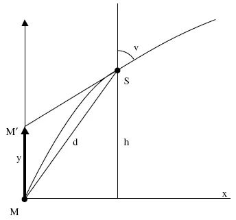
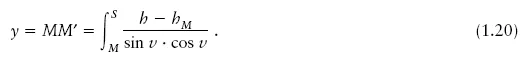
The calculation of the refraction correction can be performed in the following way: the luminous ray coming from M seems to originate from the point M′ situated on one same vertical, so that MM′ = y. One will modify the altitude of the object point M by the correction y by putting it in M′. This method of calculation has the advantage of not supposing that the axis of the acquired image is vertical, and thus works also in oblique terrestrial photogrammetry. (See Figure 1.1.4.)

Figure 1.1.4 Optical ray in the atmosphere (with a strong exaggeration of the curvature).

from where

The formula of Descartes gives us the variation of the refraction angle:

n · sin v = cte,

or dn sin v + n cos v dv = 0,

or again

In the case of photography of a zone of small extension, one will suppose the Earth to be flat, the verti...

Table of contents

• Cover Page
• Title Page
• Copyright Page
• Plates
• Contributors
• Introduction
• 1 Image acquisition. Physical aspects. Instruments
• 2 Techniques for plotting digital images
• 3 Generation of digital terrain and surface models
• 4 Metrologic applications of digital photogrammetry