Techniques of Event History Modeling

New Approaches to Casual Analysis

Hans-Peter Blossfeld, G”tz Rohwer, G"tz Rohwer

• Publisher: Psychology Press
• Year: 2001
• eBook ISBN: 9781135639112
• Topic: Psychology
• Subtopic: History & Theory in Psychology
• Index: Psychology

Including new developments and publications which have appeared since the publication of the first edition in 1995, this second edition:
*gives a comprehensive introductory account of event history modeling techniques and their use in applied research in economics and the social sciences;
*demonstrates that event history modeling is a major step forward in causal analysis. To do so the authors show that event history models employ the time-path of changes in states and relate changes in causal variables in the past to changes in discrete outcomes in the future; and
*introduces the reader to the computer program Transition Data Analysis (TDA). This software estimates the sort of models most frequently used with longitudinal data, in particular, discrete-time and continuous-time event history data.

Techniques of Event History Modeling can serve as a student textbook in the fields of statistics, economics, the social sciences, psychology, and the political sciences. It can also be used as a reference for scientists in all fields of research.

Chapter 1

Introduction

Over the last two decades, social scientists have been collecting and analyzing event history data with increasing frequency. This is not an accidental trend, nor does it reflect a prevailing fashion in survey research or statistical analysis. Instead, it indicates a growing recognition among social scientists that event history data are often the most appropriate empirical information one can get on the substantive process under study.

James Coleman (1981:6) characterized this kind of substantive process in the following general way: (1) there is a collection of units (which may be individuals, organizations, societies, or whatever), each moving among a finite (usually small) number of states; (2) these changes (or events) may occur at any point in time (i.e., they are not restricted to predetermined points in time); and (3) there are time-constant and/or time-dependent factors influencing the events.

Illustrative examples of this type of substantive process can be given for a wide variety of social research fields (Blossfeld, Hamerle, and Mayer 1989): in labor market studies, workers move between unemployment and employment,¹ full-time and part-time work,² or among various kinds of jobs;³ in social inequality studies, people become a home-owner over the life course;⁴ in demographic analyses, men and women enter into consensual unions, marriages, or into father-/motherhood, or are getting a divorce;⁵ in sociological mobility studies, employees shift through different occupations, social classes, or industries;⁶ in studies of organizational ecology, firms, unions, or organizations are founded or closed down;⁷ in political science research, governments break down, voluntary organizations are founded, or countries go through a transition from one political regime to another;⁸ in migration studies, people move between different regions or countries;⁹ in marketing applications, consumers switch from one brand to another or purchase the same brand again; in criminology studies, prisoners are released and commit another criminal act after some time; in communication analysis, interaction processes such as interpersonal and small group processes are studied;¹⁰ in educational studies, students drop out of school before completing their degrees, enter into a specific educational track, or later in the life course, start a program of further education;¹¹ in analyses of ethnic conflict, incidences of racial and ethnic confrontation, protest, riot and attack are studied;¹² in socialpsychological studies, aggressive responses are analyzed;¹³ in psychological studies, human development processes are studied;¹⁴ in psychiatric analysis, people may show signs of psychoses or neuroses at a specific age;¹⁵ in social policy studies, entry to and exit from poverty, transitions into retirement or the changes in living conditions in old age are analyzed;¹⁶ in medical and epidemiological applications, patients switch between the states “healthy” and “diseased” or go through various phases of an addiction career;¹⁷ and so on.

Technically speaking, in all of these diverse examples, units of analysis occupy a discrete state in a theoretically meaningful state space and transitions between these states can virtually occur at any time.¹⁸ Given an event history data set, the typical problem of the social scientist is to use appropriate statistical methods for describing this process of change, to discover the causal relationships among events and to assess their importance.

This book has been written to help the applied social scientist to achieve this goal. In this introductory chapter we first discuss different observation plans and their consequences for causal modeling. We also summarize the fundamental concepts of event history analysis and show that the change in the transition rate is a natural way to represent the causal effect in a statistical model. The remaining chapters are organized as follows:

• Chapter 2 describes event history data sets and their organization. Also shown is how to use such data sets with TD A.

• Chapter 3 discusses basic nonparametric methods to describe event history data, mainly the life table and the Kaplan-Meier (product-limit) estimation methods.

• Chapter 4 deals with the basic exponential transition rate model. Although this very simple model is almost never appropriate in practical applications, it serves as an important starting point for all other transition rate models.

• Chapter 5 describes a simple generalization of the basic exponential model, called the piecewise constant exponential model. In our view, this is one of the most useful models for empirical research, and so we devote a full chapter to discussing it.

• Chapter 6 discusses time-dependent covariates. The examples are restricted to exponential and piecewise exponential models, but the topic— and part of the discussion—is far more general. In particular, we introduce the problem of how to model parallel and interdependent processes.

• Chapter 7 introduces a variety of models with a parametrically specified duration-dependent transition rate, in particular Gompertz-Makeham, Weibull, log-logistic, log-normal, and sickle models.

• Chapter 8 discusses the question of goodness-of-fit checks for parametric transition rate models. In particular, the chapter describes simple graphical checks based on transformed survivor functions and generalized residuals.

• Chapter 9 introduces semi-parametric transition rate models based on an estimation approach proposed by D. R. Cox (1972).

• Chapter 10 discusses problems of model specification and, in particular, transition rate models with unobserved heterogeneity. The discussion is mainly critical and the examples are restricted to using a gamma mixing distribution.

1.1 Causal Modeling and Observation Plans

In event history modeling, design issues regarding the type of substantive process are of crucial importance. It is assumed that the methods of data analysis (e.g. estimation and testing techniques) cannot only depend on the particular type of data (e.g. cross-sectional data, panel data, etc.) as has been the case in applying more traditional statistical methodologies. Rather, the characteristics of the specific kind of social process itself must “guide” both the design of data collection and the way that data are analyzed and interpreted (Coleman 1973, 1981, 1990).

To collect data generated by a continuous-time, discrete-state substantive process, different observation plans have been used (Coleman 1981; Tuma and Hannan 1984). With regard to the extent of detail about the process of change, one can distinguish between cross-sectional data, panel data, event count data, event sequence data, and event history data.

In this book, we do not treat event count data (see, e.g., Andersen et al. 1993; Barron 1993; Hannan and Freeman 1989; Olzak 1992; Olzak and Shanahan 1996; Minkoff 1997; Olzak and Oliver 1996), which simply record the number of different types of events for each unit (e.g. the number of upward, downward, or lateral moves in the employment career in a period of 10 years), and event sequence data (see, e.g., Rajulton 1992; Abbott 1995; Rohwer and Trappe 1997; Halpin and Chan 1998), which document sequences of states occupied by each unit. We concentrate our discussion on cross-sectional and panel data as the main standard sociological data types (Tuma and Hannan 1984) and compare them with event history data. We use the example shown in Figure 1.1.1. In this figure, an individual’s family career is observed in a cross-sectional survey, a panel survey, and an event-oriented survey.

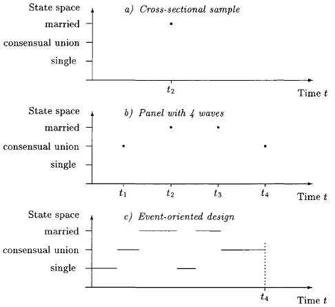
Figure 1.1.1 Observation of an individual’s family career on the basis of a cross-sectional survey, a panel study, and an event history-oriented design.

1.1.1 Cross-Sectional Data

Let us first discuss the cross-sectional observation. In the social sciences, this is the most common form of data used to assess sociological hypotheses. The family history of the individual in Figure 1.1.1 is represented in a cross- sectional study by one single point in time: his or her marital state at the time of interview. Thus, a cross-sectional sample is only a “snapshot” of the substantive process being studied. The point in time when researchers take that “picture” is normally not determined by hypotheses about the dynamics of the substantive process itself, but by external considerations like getting research funds, finding an appropriate institute to conduct the survey, and so on.

Coleman (1981) has demonstrated that one must be cautious in drawing inferences about the effects of explanatory variables in logit models on the basis of cross-sectional data because, implicitly or explicitly, social researchers have to assume that the substantive process under study is in some kind of statistical equilibrium. Statistical equilibrium, steady-state, or stability of the process means that although individuals (or any other unit of analysis) may change their states over time, the state probabilities are fairly trendless or stable. Therefore, an equilibrium of the process requires that the inflows to and the outflows from each of the discrete states be equal over time to a large extent. Only under such time-stationary conditions is it possible to interpret the estimates of logit and log-linear analyses, as demonstrated by Coleman (1981).

Even if the assumption of a steady state is justified in a particular application, the effect of a causal variable in a logit and/or log-linear model should not be taken as evidence that it has a particular effect on the substantive process (Coleman 1981; Tuma and Hannan 1984). This effect can have an ambiguous interpretation for the process under study because causal variables often influence the inflows to and the outflows from each of the discrete states in different ways. For example, it is well-known that people with higher educational attainment have a lower probability to become poor (e.g. receive social assistance); but at the same time educational attainment obviously has no significant effect on the probability to get out of poverty (see, e.g., Leisering and Leibfried 1998; Leisering and Walker 1998; Zwick 1998). This means that the causal variable educational attainment influences the poverty process in a specific way: it decreases the likelihood of inflows into poverty and it has no impact on the likelihood of outflows from poverty. Given that the poverty process is in a steady-state, logit and/or log-linear analysis of cross-sectional data only tells the difference in these two directional effects on the poverty process (Coleman 1981). In other words, cross-sectional logit and/or log-linear models can only show the net effect of the causal variables on the steady-state distribution and that can be misleading as the following example demonstrates.

Consider that we are studying a process with two states (“being unemployed” and “being employed”), which is in equilibrium (i.e. the unemployment rate is trendless over time); and let us further assume that the covariate “educational attainment” increases the probability of movement from unemployment to employment (UE → E) and increases the probability of movement from employment to unemployment (E → U...

Table of contents

• Cover
• Half Title
• Title Page
• Copyright Page
• Table of Contents
• Preface
• 1 Introduction
• 2 Event History Data Structures
• 3 Nonparametric Descriptive Methods
• 4 Exponential Transition Rate Models
• 5 Piecewise Constant Exponential Models
• 6 Exponential Models with Time-Dependent Covariates
• 7 Parametric Models of Time-Dependence
• 8 Methods to Check Parametric Assumptions
• 9 Semi-Parametric Transition Rate Models
• 10 Problems of Model Specification
• Appendix A: Basic Information About TDA
• References
• About the Authors
• Index