Briggs' Information Processing Model of the Binary Classification Task

S. Mudd

• Publisher: Psychology Press
• Year: 2019
• Print ISBN: 9780898592917
• eBook ISBN: 9781317706632
• Topic: Psychology
• Subtopic: Cognitive Psychology & Cognition
• Index: Psychology

First published in 1983. This monograph is a review of the evolution of George Briggs' informationprocessing model from a general schema beginning with the work of Saul Sternberg (1969a) and Edward E. Smith (1968) to a fairly well-detailed schematic representation of central processes that Briggs was working on at the time of his early death.

1	Basic Concepts

This chapter reviews four concepts necessary to understand the Briggs binary classification program: the information measure (H) as an empirical index versus its status as a theoretical construct; the Sternberg paradigm, particularly its logic as an experimental design; the binary character classification task (BCT); and a note on the general nature of scientific models.

THE INFORMATION MEASURE

According to Garner (1962, p. 5), a pioneer in the application of information theory and measurement to psychological problems, the selection of the binary digit, the bit, as the unit of information processing was arbitrary. The only requirement for a measure of information is that: (1) the index be monotonically related to the number of possible outcomes in a choice situation (because uncertainty increases directly with the number of possible outcomes); and (2) each additional unit on the scale represents the same amount of information (uncertainty reduction). Concerning this second requirement, a direct count of outcome possibilities does not work because, for example, going from four to five outcomes represents a change in probability of occurrence of one outcome from p = . 25 to p = .20, whereas going one unit from three to four represents an outcome probability change from p = .33 to p = .25. The single-unit increase in outcomes represents a difference in uncertainty of .05 in the first case and a difference of .08 in the second. The single- (equal) unit increment represents unequal uncertainty increments.

Any logarithmic measure has the necessary properties specified by Garner (1962), a monotonic relationship to number of outcomes and equal intervals with respect to uncertainty represented, but the particular measure, log₂, has been accepted as the standard measure of information. In the case of log₂ the doubling of the number of outcome possibilities adds one unit of uncertainty, that is, one bit. For example, an increase in number of outcomes from four to eight adds one bit of uncertainty (log₂ 4 = 2; log₂ 8 = 3). From the standpoint of uncertainty reduction, any event that reduces uncertainty by half is said to have transmitted one unit (bit) of information (i.e., ¼ = p.25; ⅛ = p.125).

To calculate the average amount of uncertainty in an array of events where the events might differ in terms of their probability of occurrence, the following formula is employed:

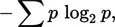(1)

or, more clearly,

(2)

Both expressions yield the average uncertainty in an array of events or, alternatively, the average information transmitted by the occurrence of a single event from that array. The second expression (2) is more easily related to the preceding discussion than (1). The term 1/p in (2), when divided through, indicates the number of outcomes associated with probability of occurrence (p) for a given event. This number is then converted to units on the log₂ scale and multiplied by p to weight that single event’s contribution to the average information in the array by the probability of that single event’s occurrence. For example, given an array of three events with the probabilities of occurrence (p) shown below, the calculations are as follows:

Event	p
1	.20	5.00	2.32	.464
2	.30	3.33	1.73	.521
3	.50	2.00	1.00	.500
				= 1.485

The term log₂ (1/p) indexes the information emitted when a particular event, for example, event 3, actually occurs. Because any event occurs only with some probability, the contribution of log₂ (1 /p₃) to the average information emitted when any of the events in the array occurs is weighted (multiplied) by p₃, the probability that “any” event in a given occurrence is, in fact, “the” event, event 3. The summation (∑) across all events in the array collects the information contribution to the array average from each event (1−3) yielding an average of 1.485 bits per event. Note that this number is the average [log₂ (1/p)] value for the three individual events when they have been properly weighted for how often they may be expected to occur (p_i). The minus sign in front of equation (1), the famous Shannon-Wiener expression, indicates that negative log values of p are involved, these values being equal to the log₂ (1/p). Tables of information values corresponding to occurrence probabilities ranging from p = .001 to .999 are usually expressed in terms of negative log values as a convenience so that entry can be made using the p value rather than its reciprocal 1 / p.

Some consideration should be given to the potential for confusion surrounding the use of the bit. The confusion arises from the implicit inference, made by many working with the binary metric, that the bit in indexing a psychological variable (e.g., response uncertainty) also represents a mathematical model of the response selection process. Garner (1962, pp. 14–15) discussed this subtle trap quite clearly. It is as though the investigator expects his measure of a variable tapping a psychological process to represent how that process operates.

A classic study by Paul Fitts (1954) on manual movement provides a good example of this problem. Fitts defined movement difficulty in informational terms (bits per response) as follows:

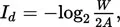(3)

where A represents the amplitude of movement between the midpoints of two targets each of width W_s; a 16-cm movement (A) between two 1-cm targets (W = 1.00 cm) would involve − log₂ (1.00/32), or 5, bits of information per response (I_d). When movement times (MT) were recorded on a group of subjects, it turned out that MT was linearly related to I_d,

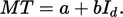(4)

This expression is one of several that have been suggested to represent the MT/I_d relationship commonly referred to as Fitts’s law. The equation [as indexed by the terms a and b in (4)] has impressive empirical validity across task types.

The problem arises when one looks beyond the descriptive statement, the empirical law, to the implications of the law for theories of movement. Theories of movement have to do with accounts of processes underlying the observed data. Now Fitts (1954) arbitrarily set the denominator of his equation at 2A because 2A “makes the index (of difficulty, I_d) correspond rationally to the number of successive fractionizations required to specify the tolerance range (W_s) out of a total range (A) extending from the point of initiation of a movement to a point equidistant on the opposite side of the target [p. 388].” The conceptual trap against which Garner (1962) warned would in this case be to accept the empirical finding, a good fit of MT to I_d, as evidence that the motor control system in fact operates by making successive bisections of the movement space in controlling arm placement. It may or it may not. Whether the I_d measure directly reflects, or models, the central motor control process must be established in the framework of other, converging experiments. At the same time there is no doubt of the validity of the empirical statement, Fitts’s law, because the general function has been replicated by other investigators.

Briggs’ measure of central processing uncertainty (H_c), to be presented later, should be considered in the same way as Fitts’ law. Justification of its use in the early Briggs reports in which (H_c) was introduced was based primarily on logical grounds, whereas his later studies were directed toward the empirical validation of (H_c). At no point was it necessary to consider (H_c) as anything more than a descriptive index of central processing uncertainty, although in later papers Briggs wrote as if the process underlying the binary classification task were in fact based on a binary search algorithm.

THE BINARY CLASSIFICATION PARADIGM

The second basic concept needed to follow the evolution of Briggs’ research program is the binary classification paradigm. In recent years the BCT has become a standard setup for cognitive research, a sort of Skinner box of cognitive psychology. And for comparable reasons: it provides an easily controlled situation for the observation of a relatively simple behavior, but a behavior that has been shown to be exquisitely sensitive to a number of meaningful psychological variables.

Although there are a number of variations on the basic task (Nickerson, 1973), the essential arrangement in binary classification is to provide subjects in the experiment with a set of stimulus items (words, numbers, faces, etc.) divisible into two categories. The two categories are defined as the positive and negative set by the experimenter who assigns stimuli to one or the other set. After receiving information about the set categories and learning which items belong to the positive and which to the negative set, the subject is presented with a series of “probes,” items from one of the two sets that he is expected to classify. Reaction times (the dependent variable) are recorded and evaluated for differences as a function of various experimental manipulations such as a positive set size, probability of occurrence of the positive set, or type of stimuli.

Observed time differences are considered to arise from corresponding differences in duration of the information-processing stages assumed to make up the sequences of events intervening between the presentation of the external stimulus (probe) and the occurrence of the overt reaction (classification response). The pattern of such observed differences allows the researcher to make inferences about the number, order, and processing characteristics of the hypothesized stages. The Sternberg additive-factor method, to be reviewed in the following section, is in effect a set of rules and guidelines for making such inferences. Before proceeding to that section, however, it is useful to review why the BCT is so widely used in the experimental analysis of cognitive processes.

Nickerson (1973, pp. 450–451) cited two major reasons why the BCT is popular among cognitive researchers, both based on the fact that research in cognition is concerned with decision, not motor, processes and with central, not peripheral, limitations on human performance. First of all, the simplicity of the binary choice response allows it to be kept constant across a great variety of experimental manipulations of cognitive variables. Such constancy allows observed differences in RT to be attributed to cognitive variables, as opposed to the invariant motor conditions. Second, that same simple nature of the binary response keeps the proportion of overall reaction time attributable to the motor component small enough that the variability associated with it does not mask response latency differences arising from the central, cognitive factors. A third reason for the popularity of the binary classification task is perhaps too obvious to mention. Nevertheless, the task as a memory task can easily be arranged to provide errorless performance. Traditional memory work very often used error scores as the dependent variable. To shift to a time measure of memory performance not only allows one to study memory processes when they are functioning properly but also provides a continuous, as opposed to a discrete (number of errors), measure of great sensitivity. The continuous property of time measures provides for the discrimination of finer differences and more subtle effects than is possible with discrete error measures.

THE STERNBERG ADDITIVE-FACTOR METHOD

The Sternberg additive-factor method is direct heir to the Helmholtz–Donders subtractive method. The logic underlying both is to make two observations under identical conditions, except for a single feature of the experiment. Observed differences in experimental outcome, given that both sets of observed conditions are otherwise identical, may then be attributed to the one feature that is different. The reasoning, of course, is the logic of the simple one-variable, two-condition experiment.

The Helmholtz-Donders Method

In Helmholtz’s classic measurement of the velocity of the nerve impulse, the dependent variable was the measured reaction time (RT) of a frog leg muscle (gastrocnemius) to an electrical stimulus delivered via a long or a short length of nerve (the independent variable). The difference in RT for the long and short lengths of nerve was attributable to the difference in length of nerve traversed by the stimulus, because all other experimental conditions were identical for both nerve lengths. By dividing the experimentally established difference in length of nerve traveled by the stimulus by the observed difference in time required to initiate the muscle contraction in the two conditions, Helmholtz accomplished what his contemporaries considered to be impossible, the measurement (centimeters per second) of the velocity of the nerve impulse (Boring, 1950, p. 41).

F. C. Donders (1969) a 19th century Dutch physiologist first applied the subtractive method to mental phenomena. In his words: “The idea occurred to me to interpose into the process of the physiological time (simple reaction time) some ...

Table of contents

• Cover
• Half Title
• Title Page
• Copyright Page
• Table of Contents
• PREFACE
• INTRODUCTION AND OVERVIEW
• 1. BASIC CONCEPTS
• 2. PHASE 1: DIFFERENTIATION OF PROCESSING STAGES
• 3. PHASE 2: SPECIFICATION OF STAGE 1 PROCESSES
• 4. PHASE 3: SPECIFICATION OF STAGE 2 PROCESSES: VALIDATION OF (Hc)
• 5. PHASE 4: ELABORATION OF THE STAGE 2 CENTRAL COMPARISON PROCESS
• 6. PERSPECTIVES ON BRIGGS’ BCT RESEARCH
• REFERENCES
• AUTHOR INDEX
• SUBJECT INDEX