Finite Element Method

Applications in Solids, Structures, and Heat Transfer

Michael R. Gosz

• Publisher: CRC Press
• Year: 2017
• Print ISBN: 9780849334078
• eBook ISBN: 9781351992039
• Topic: Technology & Engineering
• Subtopic: Applied Mathematics
• Index: Technology & Engineering

The finite element method (FEM) is the dominant tool for numerical analysis in engineering, yet many engineers apply it without fully understanding all the principles. Learning the method can be challenging, but Mike Gosz has condensed the basic mathematics, concepts, and applications into a simple and easy-to-understand reference. Finite Element Method: Applications in Solids, Structures, and Heat Transfer navigates through linear, linear dynamic, and nonlinear finite elements with an emphasis on building confidence and familiarity with the method, not just the procedures. This book demystifies the assumptions made, the boundary conditions chosen, and whether or not proper failure criteria are used. It reviews the basic math underlying FEM, including matrix algebra, the Taylor series expansion and divergence theorem, vectors, tensors, and mechanics of continuous media. The author discusses applications to problems in solid mechanics, the steady-state heat equation, continuum and structural finite elements, linear transient analysis, small-strain plasticity, and geometrically nonlinear problems. He illustrates the material with 10 case studies, which define the problem, consider appropriate solution strategies, and warn against common pitfalls. Additionally, 35 interactive virtual reality modeling language files are available for download from the CRC Web site. For anyone first studying FEM or for those who simply wish to deepen their understanding, Finite Element Method: Applications in Solids, Structures, and Heat Transfer is the perfect resource.

1

Introduction

The finite element method made its debut after a series of papers was published by Turner in 1959 [1]. Before 1965, the title, “Finite Element Method,” did not even exist; the method was referred to as the direct stiffness method (DSM). For the most part, the method was confined to the structural mechanics community and the aerospace industry. An excellent article on the history of the finite element method has been published by Felippa [2]. Since the genesis of the method during the early 1960s, thousands of articles have been published on the subject. Today, the method has reached such a state of maturity that it is now thought of as a method for solving general field problems in all areas of engineering and the physical sciences.

A modern definition of the finite element method might state that it is simply a numerical technique for obtaining approximate solutions to partial differential equations. To illustrate this idea, suppose that an engineer wants to obtain the temperature distribution in a thin plate subjected to some sort of external heat source. To accomplish this task, the engineer must make a variety of assumptions, and develop an appropriate mathematical model that is both physically realistic (retains the essential physics in the problem) and is yet amenable to solution. As an example, the engineer may assume steady-state conditions (the temperature field in the plate does not change with time), the top and bottom of the plate are perfectly insulated, the heat conduction is isotropic (the material’s resistance to heat flow is the same in all directions), etc. Under such conditions, the temperature field in the plate satisfies the two-dimensional Laplace’s equation. That is,

${\nabla }^{2}T=0$

or

$\frac{{\partial }^{2}T}{\partial X^2}+\frac{{\partial }^{2}T}{\partial Y^2}=0$

(1.1)

For simple geometries, a closed-form (analytical) solution to Laplace’s equation can be obtained; however, for complicated geometries it is usually necessary to resort to numerical techniques. The main idea in the finite element method is to discretize or “break up” the domain of interest into a collection of points and subdomains called nodes and elements. This idea is depicted in Figure 1.1. Once the domain of interest is discretized, the field variable of interest, temperature in this case, is interpolated throughout the area or volume of the element using simple polynomial interpolation functions called shape functions. Loosely speaking, for linear field problems the process of discretizing the domain into nodes and elements leads to a system of linear algebraic equations that can be readily solved on a digital computer. For nonlinear problems the technique is very much the same, except the equations are solved in an iterative manner, with each iteration solving a system of linear algebraic equations.

FIGURE 1.1
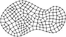
Finite element mesh.

The finite element procedure

The finite element procedure involves three general phases: a pre-processing phase, an analysis phase, and a post-processing phase. The three phases are illustrated in Figure 1.2. Perhaps the most time consuming and difficult of the three phases is the pre-processing phase. Given a physical problem of interest, the engineer must use sound judgement to transform the real-world problem into a mathematical model that captures the essential physics and is amenable to numerical solution. After making reasonable assumptions and coming up with a suitable mathematical model, usually involving a partial differential equation along with appropriate boundary conditions, he must then decide what type of analysis to perform: linear, nonlinear, transient, steady-state, etc. He must also decide upon suitable material properties, choose the appropriate type of finite element, and then create a finite element mesh that is sufficiently refined in regions where large gradients in the field variable are expected. Mesh generation by itself is a time-consuming process. Fortunately, with the advent of modern commercial pre-processing software, the amount of time spent in the pre-processing phase has been cut considerably and made easier than ever before.

For the most part, the analysis phase of the finite element procedure is like feeding the data created in the pre-processing phase into a black box. During the analysis phase, a computer program reads the data and solves a linear system of algebraic equations, either once for linear problems, or many times (often iteratively) for nonlinear and/or dynamic problems. When the analysis phase is finished, the results of interest such as nodal displacements and temperatures are output to a data file or files. Element quantities such as stress, strain, and heat flux can also be output at the user’s request.

FIGURE 1.2
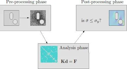
Flow chart of the finite element procedure.

In the final phase of the finite element procedure, the engineer faces the difficult task of interpreting the results of the analysis phase. The post-processing phase has been made significantly easier throughout the years through the development of user-friendly software packages with excellent graphics capabilities. The post-processing phase still, however, requires a good working knowledge of the physics of the problem of interest. For example, in a stress analysis, the engineer may want to know if a solid body under a given set of external loads will fail. To answer this question, the engineer must decide upon an appropriate failure criterion and then carefully investigate the stress fields in the solid. The engineer typically does this by observing color contour plots. At this time the engineer must assess whether or not the nice-looking contour plots make sense. In particular, he must be able to answer questions such as: Are the boundary conditions satisfied? Is the finite element mesh sufficiently refined? Was the assumption of linear material behavior appropriate? Is a more complicated analysis required?

Where do we go from here?

The finite element method is a rich and exciting subject. Learning the finite element method can be difficult, but ultimately very satisfying if we pay attention to the details of the method along the way. Let us now begin our journey in the next chapter by studying the mathematical background that is needed to obtain an excellent understanding of the finite element method. Starting the journey in this fashion may seem slow at first, but stay patient. You will be rewarded.

2

Mathematical Preliminaries

To climb steep hills requires a slow pace at first.

—Shakespeare

2.1 Matrix algebra

A matrix is a tool for arranging numerical values and/or functions in an organized manner. A matrix contains rows and columns. An element of a matrix is the number (or function) that occupies a specific row and column. As an example, consider the following matrix:

$\begin{array}{rr}\hfill A=& \hfill \left[\begin{array}{rr}\hfill 1& \hfill 3\\ \hfill 4& \hfill 2\\ \hfill 5& \hfill 6\end{array}\right]\end{array}$

(2.1)

In this example, and t...

Table of contents

• Cover
• Half Title
• Series Page
• Title Page
• Copyright Page
• Dedication
• Preface
• Table of Contents
• 1 Introduction
• 2 Mathematical Preliminaries
• 3 One-Dimensional Problems
• 4 Linearized Theory of Elasticity
• 5 Steady-State Heat Conduction
• 6 Continuum Finite Elements
• 7 Structural Finite Elements
• 8 Linear Transient Analysis
• 9 Small-Strain Plasticity
• 10 Treatment of Geometric Nonlinearities
• Bibliography
• Index