Food Toxicology

Debasis Bagchi, Anand Swaroop, Debasis Bagchi, Anand Swaroop

• Publisher: CRC Press
• Year: 2016
• ISBN:
  9781315354248
• Edition: 1
• Topic: Medicine
• Subtopic: Toxicology

Food toxicology studies how natural or synthetic poisons and toxicants in diverse food products cause harmful, detrimental, or adverse side effects in living organisms. Food toxicology is an important consideration as food supply chain is becoming more multinational in origin, and any contamination or toxic manifestation may cause serious, wide-spread adverse health effects. Food Toxicology covers various aspects of food safety and toxicology, including the study of the nature, properties, effects, and detection of toxic substances in food and their disease manifestations in humans. It will also include other aspects of consumer product safety.

The first two chapters discuss the measurement of toxicants and toxicity and the importance of dose-response in food toxicology. Additional chapters discuss the aspects of food associated carcinogenesis and food-derived chemical carcinogenesis, food allergy, pathogens associated with fruits and vegetables, and the detrimental effects of radionuclides exposure. The chapters also cover the most important heavy metal contaminants, namely mercury, lead and vanadium, and Fluoride toxicity, which is extensively discussed in its own chapter.

Toxicologists, scientists, researchers in food toxicology, nutritionists, and public health care professionals will find valuable information in this book on all possible intricate areas of food toxicology.

1	Dose–Response An Overview and Significance in Food Toxicology Lauren Connelly, Katheryne Daughtry, Jennifer Gill, Ellen Goertzen, Cameron Parsons, and Gabriel Keith Harris

CONTENTS

1.1 Introduction

1.2 Dose–Response Models: Dangerous Curves

1.3 Hormesis

1.4 Animal Models in Toxicity Testing

1.5 Codosing

1.6 Conclusion

References

1.1 INTRODUCTION

How safe is it to eat this food or this diet? This is the central question of food toxicology. To answer that simple question, we must consider the toxicity of food components, either as single components or as mixtures. We must also consider the methods used to determine toxicity. While all food components may be toxic at some level, food toxicology is primarily concerned with those that may have harmful effects at low doses. These effects may be acute (apparent after only one exposure) or chronic (effects that are only observed after repeated exposures). Acute effects would include the ingestion of bacterial toxins at a single meal, with an onset of symptoms occurring within hours or days. Chronic effects might include drinking water contaminated with arsenic, where symptoms only appear after months or years of consumption. In toxicology, something that may cause harm is referred to as a hazard. Risk is the probability of being harmed by a particular hazard. The determination of risk, better known as risk assessment, seeks to understand both the hazard and degree of exposure to it, in order to answer the “how safe is it?” question. Dose–response experiments involving cell culture and animal models are a key component of risk assessment: the estimation of how safe or unsafe a food might be. While the use of animals is viewed as essential in toxicology today, it raises controversy and questions about how well experimental results apply to humans. Our diets, the food we choose to eat on a daily basis, may be the ultimate dose–response experiment, since we eat and drink mixtures of thousands of compounds each day, each with a different toxic dose.

The Renaissance physician Paracelsus (1493–1541), often referred to as the Father of Toxicology, proposed the concept that “the dose makes the poison” (Borzelleca, 2000). This means that everything is toxic at a sufficiently high dose. For this reason, toxicologists do not ask whether or not something is toxic. Instead, they ask questions like “How toxic is this substance?” or “How risky is it?” Materials that most of us would consider poisons, such as arsenic, cyanide, or botulinum toxin, can cause harm or death at very low doses. For example, it has been estimated that 1 g, or less than onequarter teaspoon, of botulinum toxin would be sufficient to kill one million people (Arnon, 2001). On the other end of the toxicity spectrum, even pure water can cause harm or death if an adult were to drink about 6 L (nearly 2 gal) in a period of several hours. The result of consuming too much water is called hyponatremia (low blood sodium), an osmotic imbalance that can cause brain swelling, seizures, and death (Farrell and Bower, 2003; Dolan et al., 2010). Since all food ingredients, including nutrients, may cause harm at some level, it is important to define these levels and remain well below them to avoid harming even sensitive individuals.

This chapter deals with dose–response, so it is important to define dose. When taking a “dose” of aspirin or other medications, it is common to think in terms of an amount, such as a tablet containing a certain number of milligrams of active compound. In toxicology, dose is typically defined as a concentration of a substance. Concentrations are ratios of mass to mass, mass to volume, or volume to volume. Substances may be quantified in terms of milligrams per kilogram (otherwise known as parts per million), grams per kilogram, grams per liter, etc. Why not just use an amount like 5 g or 20 mL? The reason is that variability in body weight, body composition, and metabolism affects how compounds distribute through the body. A small child may react very differently to the same 5 g of material than an adult. Part of this is due to age-based differences in metabolism, but a large component is due simply to differences in dilution factors between the child’s smaller volume and the adult’s larger volume. In this way, concentration is a more effective measure of dose than mass or volume alone. The term dose–response refers to the effect that a given concentration of a chemical substance has on the body in general or on specific target organs. These effects could be beneficial (as in the case of an appropriate dose of a medicine) or harmful (as in the case of a poison). Although dose–response relationships have been studied since the 1500s, there remains a vast amount of information yet to be learned. While toxicologists agree that the “dose makes the poison,” debate continues about the relationship between the dose and the response. Is it linear, meaning that any dose causes some harm? Is there a threshold dose, below which no harm occurs for all toxins? Can tiny doses of toxic materials be beneficial? Why are some individuals especially sensitive to certain food components? What is the effect of consuming a mixture of many compounds (as with single foods or whole diets) instead of just one? This chapter seeks to address these questions by examining dose–response relationships in food.

1.2 DOSE–RESPONSE MODELS:
DANGEROUS CURVES

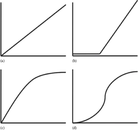
Like other scientific disciplines, food toxicology attempts to understand the natural world using models, or simplifications of reality. This is a practical necessity since it is physically and financially impossible to study all hazards in all foods for all people. The shape of dose–response curves is essential to the understanding of a substance’s toxicity (Calabrese et al., 1999 and Calabrese, 2003). While dose–response is typically curvilinear, it may be described in terms of either linear or nonlinear models, where dose appears on the x-axis and response appears on the y-axis. In the case of toxicology, the response may be harm or death. Linear models may result from examining only the linear portion of a dose–response curve, from linear extrapolation, or from data transformations designed to linearize a curve. Despite their limitations, linear models are preferred because of their ease of analysis and interpretation. Figure 1.1a shows a linear dose–response curve. This type of linear model assumes that there is no safe dose for a given substance and that any dose will cause some harm. These types of linear models are used to estimate risk related to cancer-causing agents (carcinogens), giving an added margin of safety. Threshold models (Figure 1.1b) assume that no harm occurs below a certain dose, but that there is a linear increase in harm after a threshold dose is surpassed. This threshold dose is referred to as “no observed adverse effect level” (NOAEL). The NOAEL could be thought of as the highest safe dose. NOAELs can be determined for either acute or chronic exposures of the same compound (the dose will be different for each type of exposure).

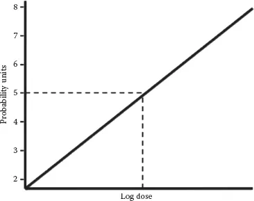
Most dose–response relationships in food toxicology are not linear. Plotting dose versus percent response for a sufficiently large population results in a curvilinear plot (Figure 1.1c). Dose is typically converted to a log scale, resulting in a sigmoid curve (Figure 1.1d). This conversion makes the center portion of the plot more linear, allowing for the determination of three important dose levels, the NOAEL, mentioned previously, the LOAEL, and the LD50. The LOAEL is the “lowest observed adverse effect level.” The LOAEL is the lowest unsafe dose, or the minimum dose at which observable harm occurs. The LD50, or median lethal dose, describes the level at which 50% of a test population dies. LD50 testing is done in animal models and then extrapolated to humans, typically on a milligram per kilogram dose basis. Several species may be tested to estimate the human LD50. Animal to human extrapolations are typically made based on the most sensitive species. The LD50 is one of the most common ways of making direct “apples to apples” comparisons of the toxicity of different compounds. Probit (probability unit) transformations (Figure 1.2) are used to convert sigmoidal dose–response curves to straight lines, further easing LD50 calculations. This is accomplished by replacing percentage values on the y-axis with probit values ranging from two to eight. These probit values result from adding five to the three standard deviation units above and below the dose at which 50% of the population responds. Given the assumption of a Gaussian (bell curve) distribution of responses (Figure 1.3), the probit scale would cover dose–responses for 99.7% of a given population. On this scale, the LD50 is the dose corresponding to a probit value of five (0 + 5 = 5), since the mean, by definition, has a standard deviation of zero (Deshpande, 2002). Regarding the LD50, why would half a population die and the other half survive if given the same dose of a toxin? The reason for this is that, within a given population, there are individuals that are very susceptible to the toxin, individuals who are very resistant to the toxin, and everyone else in between. Susceptibility or resistance to particular toxins may result from genetic differences in drug-metabolizing enzymes, nutritional status, age, or other factors. When considering acute versus chronic exposures, there are different NOAELs, LOAELs, and LD50s for a given compound.

FIGURE 1.1 Dose–response curve shapes before and after transformation: (a) linear model, (b) threshold model, (c) curvilinear model, and (d) sigmoid curve. The x-axes represent dose (log dose in the case of the sigmoid curve). The y-axes represent response.

FIGURE 1.2 Probit transformation to convert sigmoid curves to linear responses. The x-axis represents log dose. The y-axis represents probit (probability unit) values.

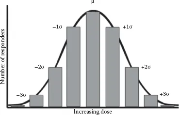
FIGURE 1.3 Gaussian distribution showing typical effects of increasing dose on the number of responders in a population, including mean dose and doses up to three standard deviations above or below the mean. Susceptible individuals may respond at doses up to three standard deviations below the mean. Resistant individuals may only respond at doses up to three standard deviations above the mean.

Since even nutrients such as vitamins and minerals may become toxic at very high levels, it is necessary to establish both upper and lower limits for their use. For essential nutrients, potential deficiencies and toxicities are estimated relative to dietary reference intakes. Dietary reference intakes take three different nutrient levels into account: estimated average requirements, recommended dietary allowances, and acceptable upper intake levels (USDA, 2010; DRIs, 2016). The recommended dietary allowances are calculated from estimated average requirements and represent intakes with two standard deviations above estimated average requirements, assuring that most of the population receives a sufficient level of essential nutrients but remains well below toxic levels. Acceptable upper intake levels correspond to the NOAELs described earlier (Taylor, 2008). Consuming more than the acceptable upper intake levels of a nutrient increases the risk of toxic effects.

For nonnutrient compounds, acceptable and tolerable daily intakes are used instead of dietary reference intakes. Acceptable daily intakes are defined as the amount of a food additive (based on a 60 kg average body weight) that can be safely consumed for a lifetime (Agget et al., 2015). Regarding food additives, an ongoing area of research is the investigation of possible links between artificial colors and attention-deficit disorder in children. While reactions have been reported when single doses of 50–100 mg have been administered in controlled trials, the question remains whether the doses normally consumed by children (reported to be approximately 60 mg per day in the United States) reach those levels (Stevens et al., 2013). Tolerable daily intakes are the amounts of nonnutrient, nonfood additive compounds that can be consumed over a lifetime without harm to the individual. Acceptable and tolerable daily intake values are generated from NOAELs based on the most sensitive species using a 100-fold margin of safety factor (Nasreddine and Parent-Massin, 2002).

Recently, the concept of linear and sigmoidal dose–response relationships has been called into question. An accumulating weight of evidence indicates that certain substances may produce nonmonotonic responses, meaning that higher doses do not uniformly produce greater effects. Examples of nonmonotonic curves would include those related to low-dose effects and to hormesis. Low-dose effects refer to the idea that compounds may produce very different effects at low doses than at high doses. Endocrine disruptors are compounds that interfere with the body’s natural hormonal balance. Bisphenol A, a breakdown product of certain plastics, exerts estrogenic effects, even at very low doses. This could result in reproductive problems and may promote hormone-sensitive cancers. Endocrine disruptors are of great interest to toxicologists because they produce responses at very low concentrations and because responses are typically nonlinear (Vandenberg et al., 2012).

1.3 HORMESIS

One final set of nonlinear curves to consider are the J-shaped and U-shaped curves related to hormesis (Figure 1.4a and b). There is a large body of literature supporting the concept that low doses of otherwise toxic compounds can have beneficial effects. This concept is referred to as “hormesis.” Dose–response curves may take on a J-shape or an inverted U-shape, depending on the endpoints measured. Generally speaking, J-shaped curves have some type of risk on the y-axis, such that risk decreases to a certain point as dose increases but then goes back up. The dose–response relationship between alcohol and stroke is an example of a J-shaped curve. Stroke risk drops as alcohol intake increases from zero to two or three drinks (one drink being defined as one ounce of alcohol) per day (Andréasson, 1998). From this perspective, two or three servings of alcohol per day appear to protect against stroke. When between four and five drinks per day are consumed, stroke risk is on par with that of nonconsumers. Beyond five drinks per day, stroke risk dramatically increases above that observed for both nonconsumers and moderate consumers of alcohol. This means that the risk of stroke is similar for those consuming either zero or five servings of alcohol per day. From a more general perspective, the concept of the J-shaped curv...