A Laboratory Manual in Biophotonics

Vadim Backman, Adam Wax, Hao F. Zhang

• Publisher: CRC Press
• Year: 2018
• ISBN:
  9781498744331
• Edition: 1
• Topic: Medicine
• Subtopic: Biotechnology in Medicine

Biophotonics is a burgeoning field that has afforded researchers and medical practitioners alike an invaluable tool for implementing optical microscopy. Recent advances in research have enabled scientists to measure and visualize the structural composition of cells and tissue while generating applications that aid in the detection of diseases such as cancer, Alzheimer's, and atherosclerosis. Rather than divulge a perfunctory glance into the field of biophotonics, this textbook aims to fully immerse senior undergraduates, graduates, and research professionals in the fundamental knowledge necessary for acquiring a more advanced awareness of concepts and pushing the field beyond its current boundaries. The authors furnish readers with a pragmatic, quantitative, and systematic view of biophotonics, engaging such topics as light-tissue interaction, the use of optical instrumentation, and formulating new methods for performing analysis. Designed for use in classroom lectures, seminars, or professional laboratories, the inclusion and incorporation of this textbook can greatly benefit readers as it serves as a comprehensive introduction to current optical techniques used in biomedical applications.

• 
  
  

• Caters to the needs of graduate and undergraduate students as well as R&D professionals engaged in biophotonics research.

• 
  
  

• Guides readers in the field of biophotonics, beginning with basic concepts before proceeding to more advanced topics and applications.

• 
  
  

• Serves as a primary text for attaining an in-depth, systematic view of principles and applications related to biophotonics.

• 
  
  

• Presents a quantitative overview of the fundamentals of biophotonic technologies.

• 
  
  

• Equips readers to apply fundamentals to practical aspects of biophotonics.

1

General Introductory Topics

Part 1: Fundamental Mathematics

Here, we introduce basic concepts in mathematics and statistics that will be useful in the coming chapters and experiments. The content is very limited and serves only to remind readers what should be known prior to continuing. For more detailed explanations and derivations, please refer to subject matter textbooks that focus on those topics.

Dirac Delta Pulse

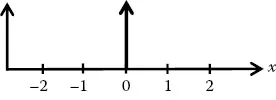
There is often a need to consider the effect on a system by a forcing function that acts for a very short time period, such as a “kick” or an “impulse.” Such an impulse is called the Dirac delta (δ) pulse, shown in Figure 1.1, and is defined as

δ(x)={+∞,x=00,x≠0	(1.1)

Figure 1.1

Dirac delta pulse.

Furthermore, the delta pulse satisfies an identity constraint:

∫−∞+∞δ(x)dx=1	(1.2)

The Dirac delta is not a function, as any extended-real function that is equal to zero everywhere except one single point cannot have a total integral of 1. While it is more convenient to define the Dirac delta as a distribution, it may be manipulated as though it were a function, thus conferring its many properties and characteristics.

The Dirac delta can be scaled by a nonzero scalar α:

∫−∞+∞δ(αx)dx=∫−∞+∞δ(u)du|α|=1|α|	(1.3)

sothatδ(αx)=δ(x)|α|	(1.4)

The Dirac delta is symmetrical and follows an even distribution such that

δ(−x)=δ(x)	(1.5)

The Dirac delta exhibits a translation property where the integral of a pulse delayed by d returns the original function evaluated at d shown by

∫−∞+∞f(x)δ(x−d)dx=f(d)	(1.6)

This is also called the sifting property of the delta pulse, as it “sifts out” the value f(d) from the function f(x). Although the integral here ranges x = ±∞, the same result is obtained for any integral bounds α and β provided that α ≤ d ≤ β.

Convolving a function f(x) with a delta pulse delayed by d has the effect of also time-delaying f(x) by d:

(f(x)∗δ(x−d))=∫−∞+∞f(τ)⋅δ(x−d−τ)dτ,	(1.7)

which gives

∫−∞+∞f(τ)⋅δ(τ−(x−d))dτ=f(x−d)	(1.8)

If f(x) is a continuous function that vanishes at infinity, the following integral evaluates to 0:

∫−∞+∞f(x)δ(x)dx=[f(x)H(x)]−∞+∞−∫−∞+∞f′(x)H(x)dx,	(1.9)

which evaluates to

−∫0+∞f′(x)dx=[−f(x)]0+∞=0.	(1.10)

Here, H(x) is the Heaviside step function whose derivative is the Dirac delta pulse.

Kronecker Delta Pulse

Similar to the Dirac delta, the Kronecker delta is represented by an impulse that equals 1 at zero and zero everywhere else. The Kronecker delta is frequently denoted by δi to distinguish it from the Dirac delta pulse.

Kronecker Comb

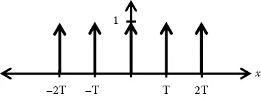
If a series of equally spaced impulses of amplitude 1 were delivered to a system (such as in the case of discrete sampling), we can see a periodic construction of Kronecker delta pulses known as a Kronecker comb.

ΔT(t)=def∑k=−∞∞δi(t−kT)	(1.11)

where δi(x) is the Kronecker delta, and T represents a given period between successive pulses. Figure 1.2 shows a graphical representation of the Kronecker comb.

Figure 1.2

Kronecker comb.

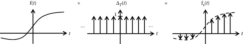
Notice that the Kronecker comb multiplied by any function f(t) would depend on f(t) only at the locations of the Kronecker pulses; hence, f(t) is “sampled” and is commonly referred to as the sampling function in cases of signal processing and electrical engineering disciplines. In Figure 1.3, this sampling process is shown for an arbitrary curve.

Figure 1.3

Piecewise sampling of f(t) via combination with Kronecker comb ΔT(t).

sinc Function

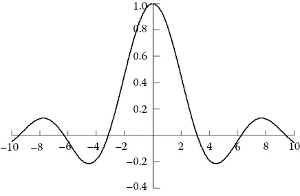
Since the Dirac delta pulse is not defined as a function, it is typically constructed by taking a limit on a function. An example of this is by using the sinc function. This function, shown in Figure 1.4, is defined as

sinc(x)=sinxx	(1.12)

Figure 1.4

Sinc function.

To construct the pulse, let

F(x)=sinc(x/a)a,	(1.13)

asa→0andF(x)→δ(x)	(1.14)

Exercise: Show that F(x) = (sinc(x/a))/a→δ(x) when a→0 in MATLAB®. Let x = −10:0.001:10 and a = 10, 1, 0.1, 0.01 and note how F(x) approaches the Dirac delta pulse.

Convolution

Convolution is a mathematical operation on two functions that gives the amount of overlap of the first function as it translates through the second. This operation is denoted with an asterisk:

(f∗g)(t)=def∫−∞∞f(τ)g(t−τ)dτ	(1.15)

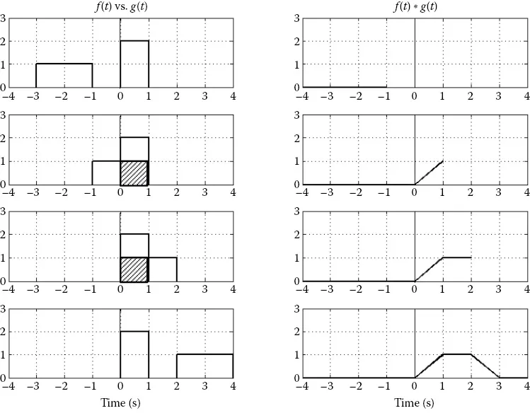
Note that convolution is commutative, so (f * g)(t) = (g * f)(t). Convolution is useful for calculating a moving average and is therefore used extensively in image and signal filtering. A visual representation of convolution is shown in Figure 1.5.

Figure 1.5

Convolution of two square impulses, one stationary and one moving along the positive x-direction. The shaded area is correspondingly plotted as the convolution result.

Cross-Correlation

Cross-correlation represents an important signal processing tool, which provides a measure of similarity between two signals. This si...