Space Weather Fundamentals

George V. Khazanov, George V. Khazanov

• Publisher: CRC Press
• Year: 2016
• ISBN:
  9781315351469
• Edition: 1
• Topic: Scienze biologiche
• Subtopic: Scienza generale

Space weather is one of the most significant natural hazards to human life and health. Conditions of the sun and in the solar wind, magnetosphere, ionosphere, and thermosphere can influence the performance and reliability of space-borne and ground-based technological systems. If conditions in the space environment are adverse, they can cause disruption of satellite operations, communications, navigation, and electric power distribution grids, leading to a variety of socioeconomic losses.

This book provides an overview of our current knowledge and theoretical understanding of space weather formation and covers all major topics of this phenomena, from the sun to the Earth's ionosphere and thermosphere, thus providing a fully updated review of this rapidly advancing field. The book brings together an outstanding team of internationally recognised contributors to cover topics such as solar wind, the earth's magnetic field, radiation belts, the aurora, spacecraft charging, orbital drag and GPS.

I

Space Weather Drivers

CHAPTER 1

The Sun

Judith Karpen and Spiro Antiochos

CONTENTS

1.1 Introduction

1.1.1 Solar Variability: The Dynamo

1.1.1.1 The Solar Cycle

1.1.1.2 Flux-Transport Dynamos

1.1.1.3 Mean-Field Dynamos

1.1.2 Slow Drivers of Space Weather

1.1.2.1 Global-Scale Magnetic Structures and Solar Wind

1.1.2.2 Local-Scale Magnetic Structures (ARs)

1.1.3 Explosive Drivers of Space Weather

1.1.3.1 Flares: Impulsive Electromagnetic and Particle Radiation

1.1.3.2 CMEs: Impulsive Mass and Magnetic-Field Driving

1.1.4 Future Prospects

Acknowledgments

References

1.1 INTRODUCTION

The Sun is the ultimate source of all space weather in the solar system. Specifically, the stressing of the Sun’s magnetic field by plasma motions from the deep interior through the photosphere, its visible surface, transfers the energy generated by fusion from the core to the plasma and magnetic field of the solar corona. Both slow and fast drivers of space weather originate in the corona, then propagate and evolve throughout the heliosphere. In this chapter, we will discuss the primary phenomena driving space weather on long (day-to-month) and short (seconds-to-minutes) timescales, and the associated mechanisms of radiative and mechanical forcing. Slow drivers include corotating interaction regions in the solar wind, which originate at the interface between closed and open magnetic flux on the rotating Sun. On similar timescales, the emergence and evolution of solar active regions (ARs), localized regions of strong magnetic flux that wax and wane with the solar cycle, cause significant fluctuations of emissions across the electromagnetic spectrum; enhancements in UV radiation and X-rays are particularly relevant to space weather because of their profound impact on planetary ionospheres. Explosive energy release in the corona, commonly ascribed to magnetic reconnection, produces massive eruptions of magnetic field and plasma (coronal mass ejections; CMEs) as well as intense bursts of electromagnetic radiation and energetic particles (flares). This impulsive activity generates the most destructive space weather events in the heliosphere, with complex consequences for planetary magnetospheres, ionospheres, neutral atmospheres, and life and technology in space and on planetary surfaces. We will describe the key observed features and fundamental physical processes leading to slow and fast variations in the Sun’s radiative, mass, magnetic, and energetic particle outputs, and point out gaps in our understanding that must be addressed by future observations, theory, and modeling.

1.1.1 Solar Variability: The Dynamo

The fundamental origin of all space weather is the variability of the Sun’s magnetism. This variability is readily apparent in both the spatial and temporal properties of the solar magnetic field. In terms of spatial properties, the most important feature of the Sun’s magnetism that leads to space weather is that the field exhibits a complex, multipolar flux distribution, very different than that of Earth’s simple dipole.

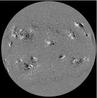
Figure 1.1 shows the line-of-sight magnetic flux at the solar surface, the photosphere, during a period of strong solar activity. The structure of the observable flux consists of a myriad of concentrations over a large range of spatial scales. Detailed analysis has shown that the number of flux concentrations exhibits a power-law dependence on spatial scale, N~Φ^−1.85, over five orders of magnitude or more (Parnell et al. 2009). All these scales may play an important role in the observed solar activity, but for space weather, the most important flux scales are likely to be the global dipolar field of the Sun and the strong concentrations of flux in sunspots with field strengths of 2000 G or more. Sunspots tend to cluster in groups to form so-called active regions (ARs), with spatial scales of order hundreds of Mms. Large complex ARs are the sites of the most energetic form of solar activity, the giant eruptions of magnetic field and plasma known as coronal mass ejections (CMEs)/eruptive flares. For the science of space weather, therefore, understanding the formation of AR magnetic fields and their dynamics in the corona and heliosphere is of paramount importance.

FIGURE 1.1 Image from the HMI magnetograph on SDO showing the positive (white) and negative (black) line-of-sight magnetic flux at the solar photosphere on January 5, 2013.

The temporal variability of the field can roughly be considered as having three dominant scales. The shortest scale is given by the characteristic wave travel time in the corona: τ ~ L/V_A, where VA is the coronal Alfvén speed. Using typical values for length scales of 100 Mm and V_A ~ 1 Mm s⁻¹ yields a timescale of order 100 s, which is the observed timescale for explosive events such as flares and CMEs. Solar activity on these timescales is discussed in Section 1.1.3. The second temporal scale is that of the period for solar rotation, ~27 days. The rotation drives recurring phenomena such as solar UV variability as ARs rotate from front to back on the disk, and the interaction of fast and slow solar wind streams in the heliosphere. This latter process is highly important for space weather, and will be discussed in detail in Chapter 2. The third timescale, which we will now discuss, is that of the solar cycle, of order a decade or so.

1.1.1.1 The Solar Cycle

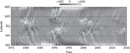
It has been known for well over a century (Schwabe 1844) that the appearance of ARs on the Sun is cyclic with a period of roughly 22 years. Figure 1.2 from Hathaway (2015) shows the salient features of the solar magnetic cycle. The daily longitudinally averaged magnetic field as observed by both ground and spacebased magnetographs is plotted for the past 30 years. It should be noted that the measurements at the poles are subject to considerable errors due to foreshortening; however, most of the structure in the field, such as ARs, is at lower latitudes. The cycle “begins” with bipolar ARs emerging at intermediate latitudes ~30° with a small latitudinal tilt to the bipoles; for example, in cycle 22 beginning in 1986, the AR bipoles in the north had a “leading” polarity (i.e., closer to the equator) that is negative while the leading polarities in the south were positive. Note that, when the cycle begins, the polar field in each hemisphere has the same sign as the leading AR polarities, while the trailing polarities, which are at slightly higher (~5°) latitude, have a polarity opposite to that of their respective pole. The cycle continues with ARs emerging at successively lower latitudes over the course of a decade or so. After emerging, the trailing polarities undergo a so-called rush to the poles, thereby, canceling the leading polarity of previously emerged ARs and eventually reversing the sign of the polar field. This process can be seen in Figure 1.2 as the broad swaths of color stretching from the AR belt to the poles. AR emergence appears to die out when the emergence reaches the equator and, subsequently, the Sun enters a phase of solar activity minimum lasting a year or two before the new cycle ARs start their emergence again at high latitudes.

FIGURE 1.2 Longitudinally averaged line-of-sight magnetic field at the solar surface. White corresponds to positive polarity and black to negative. (From Hathaway, D.H., Living Rev. Solar Phys., 12, 4, 2015.)

Two important features of the solar cycle are apparent in Figure 1.2. Even though only approximately four cycles are shown, it is evident the cycles can vary considerably in strength and in duration. In particular, we note that the present cycle, number 24, is weak (low number of ARs) and was preceded by a long minimum, the so-called deep minimum (e.g., Russell et al. 2010). In fact, the minima sometimes appear...