Air Pollution and Human Health

Lester B. Lave, Eugene P. Seskin

• Publisher: RFF Press
• Year: 2013
• Print ISBN: 9781617260582
• eBook ISBN: 9781135996734
• Topic: Biological Sciences
• Subtopic: Ecology
• Index: Biological Sciences

Upon competition of a ten year research project which analyzes the effect of air pollution and death rates in US cities, Lester B. Lave and Eugene P. Seskin conclude that the mortality rate in the US could shrink by seven percent with a similar if not greater decline in disease incidence if industries followed EPA regulations in cutting back on certain pollutant emissions. The authors claim that this reduction is sufficient to add one year to average life expectancy. Originally published in 1977.

Section II
Cross-sectional analysis of U.S. SMSAs, 1960, 1961, and 1969

Chapter 3
Total U.S. mortality, 1960 and 1961

Sections II and III will explore the empirical association between air pollution and health status (as measured by mortality). Much of the analysis will focus on whether the empirical evidence is consistent with a causal relationship. At the same time, a major output of the analysis will be a quantitative estimate of the dose-response relationship between air pollution (as measured primarily by sulfates and suspended particulates) and mortality.

The second hypothesized relationship between air pollution and mortality, discussed in chapter 1, was that long-term exposure to low levels of pollution adversely affects health. Two different types of analyses might be used to explore this hypothesis. The first would involve an investigation of a measure of health status across areas having different qualities of ambient air. The second would involve an analysis of a measure of health status within a single location experiencing changing air quality over a period of time. Of the two, it seems likely that one would observe larger differences in air quality across different places than within a single place over time. Thus, cross-sectional analysis of areas with differing pollution levels at a given time offers a greater possibility of isolating pollution effects should they exist.

Specifically, this chapter is based on analysis of annual cross-sectional data for 117 SMSAs in the United States.¹ We have sought to avoid the more obvious fallacies associated with comparing urban and rural places by using these large metropolitan areas as our units of observation. The statistical method used to analyze these data is linear multivariable regression analysis. We begin by reporting analyses of total mortality, using socioeconomic variables to control for population density, racial composition, age distribution, income, and population. Air pollution will be represented by the measured levels of sulfates and suspended particulates.²

Method

Since we had little a priori knowledge as to which measures of air pollution or which socioeconomic variables would be important, many were used in the analysis. In Equation 3.1 the total 1960 mortality rate was regressed on socioeconomic and air pollution variables across 117 SMSAs.³

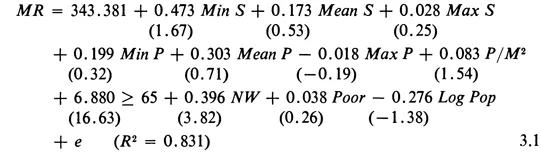
where MR is the total mortality rate in the area, Min S, Mean S, and Max S are the smallest, the arithmetic mean, and the largest, respectively, of the twenty-six biweekly sulfate readings; Min P, Mean P, and Max P are the smallest, the arithmetic mean, and the largest, respectively, of the twenty-six biweekly suspended particulate readings; P/M² is the population density in the SMSA; — 65 is the percentage of the SMSA population aged sixty-five and older; NW is the percentage of the SMSA population who are nonwhite; Poor is the percentage of the SMSA families with incomes below the poverty level; Log Pop is the logarithm of the SMSA population;⁴ and e is an error term. The scaling of the variables is reported in table D.1 (pages 321-324), along with their means and standard deviations. The figures shown in parentheses below the regression coefficients are the t statistics. Table 3.1 also reports the sums of elasticities about the mean. Each elasticity is equal to 100 × b (X/Y), where b is the estimated coefficient and X and Y are the means of the independent and dependent variables, respectively.

The results are encouraging in that more than 83 percent of the variation in the total mortality rate across these 117 SMSAs was accounted

TABLE 3.1. Total Mortality Rates, 1960

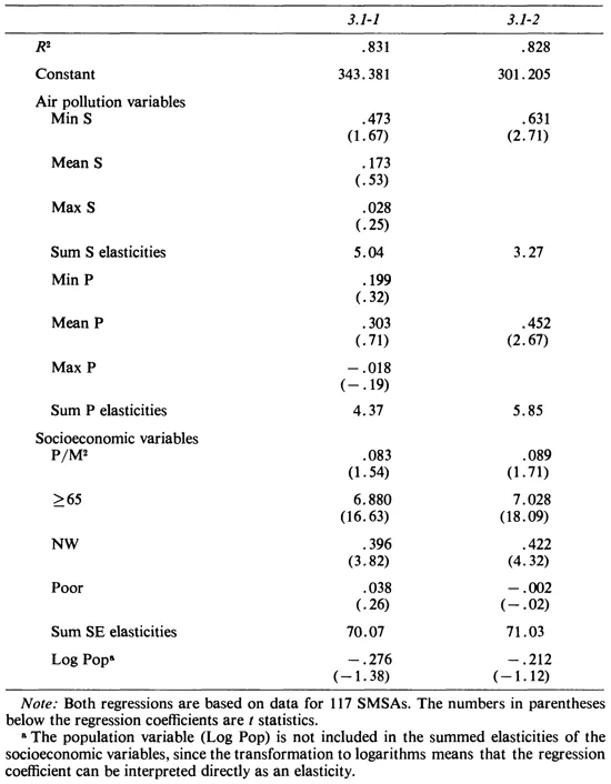
for by the eleven independent variables (R² = 0.831). The estimated coefficients for the air pollution variables were disappointing in that none had a statistically significant coefficient,⁵ and one coefficient was negative;

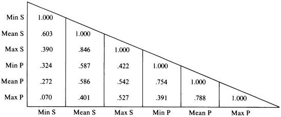
FIG. 3.1. Air pollution correlation matrix for 1960.

however, the six variables made a statistically significant contribution as a group.⁶ These results are partially explained by the high correlation between the six measures of air pollution, as is shown in figure 3.1. Such multicollinearity has the effect of increasing the standard errors of the estimated coefficients and of impairing the accuracy with which individual coefficients can be estimated. A more complete discussion of this regression appears below.

One conventional approach to regression estimation involves dropping superfluous variables in order to derive an equation which contains coefficients with predicted signs, plausible magnitudes, and statistical significance. Since our interest was centered on the air pollution variables, we initially retained only those whose coefficients were positive and exceeded their standard errors, with the further constraint that at least one sulfate measure and one particulate measure were retained. In reestimating the relationship, we often found that the retained air pollution variables were now significant (which is not surprising, since the pollution variables were highly correlated). Sometimes the retained air pollution variable contributed little to the statistical significance of the regression. Such variables were eliminated, subject to the restriction that at least one air pollution variable be retained in the final equation. This technique was used throughout our analyses of other mortality rates. (The five basic socioeconomic variables were retained throughout.) Because these relations are estimated ad hoc, they must be viewed with care.

Equation 3.1, containing all six pollution variables, is reported in table 3.1 as regression 3.1-1. (Note that all regressions are numbered according to the table in which they appear.) Regression 3.1-2 represents a similar specification but includes only the two most significant air pollution variables (Min S and Mean P). As expected, there was little loss in explanatory power when the other four measures of air pollution were deleted [R² decreased from 0.831 to 0.828; the F statistic (F = 0.40) computed to examine this loss confirmed the nonsignificance of it]. Each of the coefficients of the two remaining air pollution variables was statistically significant and approximately equal in magnitude to the sum of the three variables it represented.

Principal Component Analysis

A less-arbitrary procedure for reducing the size of the equation was also examined. As shown in figure 3.1, the six air pollution measures tended to be highly correlated. One method for circumventing the collinearity problem is to perform a principal component analysis on the pollution variables and to replace the pollution measures with the resulting components in the regressions.⁷ We have explored this method with the 1960 data. First, we found the principal components of all six pollution measures; then we found the principal components of the suspended particulate and sulfate measures separately (table 3.2). The first principal component explained 59.5 percent of the variation in the six variables, 74.8 percent of the variation in the sulfate measures, and 76.8 percent of the variation in the suspended particulate measures. The corresponding figures for the first two components together were 78.3 percent, 96.1 percent, and 97.1 percent, respectively.

Four regressions are reported in table 3.2 for the total 1960 mortality rate. Regression 3.2-1 used the original six air pollution variables and is shown for comparison; regression 3.2-2 used the two most significant air pollution variables; regression 3.2-3 used the first two principal components extracted from all six pollution measures; and regression 3.2-4 used the first two principal components from the separate analyses of the sulfate and suspended particulate measures. In addition to these components, the five socioeconomic variables were included.

Comparing regression 3.2-2 with regressions 3.2-3 and 3.2-4, one notes little or no difference between using the principal components and using the ad hoc method of selecting pollution variables. The statistical significance of the principal components of the air pollution variables was virtually

TABLE 3.2. Principal Componenets Analysis of Total Mortality Rates, 1960

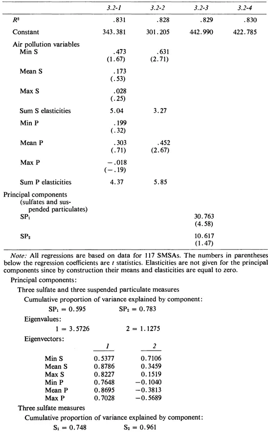
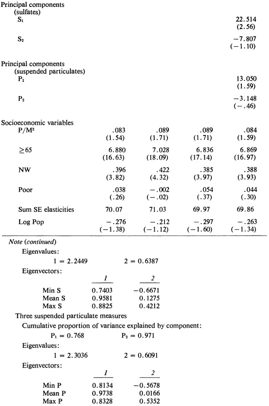
identical to the significance of the air pollution variables when they were used. The coefficients of the socioeconomic variables and their statistical significance were essentially unchanged. Thus, we concluded that little would be gained by using the principal components in place of the air pollution variables. On the contrary, interpretation of the principal components is somewhat more difficult than interpretation of the untransformed pollution measures.

Implications of the Regressions

Because there is no diagnostic problem and little or no reporting problem involved, the mortality data for total deaths are more accurate and complete than data for any of the subcategories. Thus, an analysis of total mortality is a good place to begin our study, and it serves as a reference point for analyses of other data sets. It should be noted, however, that the accuracy and completeness of these data come at some cost because they are so aggregated.⁸ Age-specific analysis is needed if the effect of air pollution on life expectancy is to be calculated;⁹ it is also desirable to determine which particular diseases are associated with air pollution. Disease-specific mortality rates are analyzed in chapter 4.

The estimates from a multivariable regression are not to be taken as proof of causation, but as evidence of associations that may or may not indicate a causal relation. Thus, we will speak of the association between a single variable, such as suspended particulates, and the mortality rate, holding other factors constant. These are not statements of causation, but are merely indications of the magnitude of the observed association.

In regression 3.1-1 (see Equation 3.1) the total mortality was regressed on all of the air pollution and socioeconomic variables. The multicollinearity among the air pollution variables and the resulting nonsignificance of the estimated coefficients make their interpretation somewhat difficult. In regression 3.1-2, only the most significant sulfate and suspended particulate measures were retained.

Over 83 percent of the variation was accounted for by the eleven independent variables in regression 3.1-1. As expected, the most significant variable was the percentage of the population aged sixty-five and older (^±65). The implication of the estimat...

Table of contents

• Cover
• Title
• Copyright
• Original Title
• Original Copyright
• Contents
• Foreword
• Preface
• Acknowledgments
• SECTION I. BACKGROUND AND THEORETICAL FRAMEWORK
• SECTION II. CROSS-SECTIONAL ANALYSIS OF U.S. SMSAs, 1960, 1961, AND 1969
• SECTION III. ANNUAL AND DAILY TIME-SERIES ANALYSIS
• SECTION IV. POLICY IMPLICATIONS
• References
• SECTION V. APPENDIXES
• Author Index
• Subject Index