Capacitance Spectroscopy of Semiconductors

Jian V. Li, Giorgio Ferrari, Jian V. Li, Giorgio Ferrari

• Publisher: Jenny Stanford Publishing
• Year: 2018
• ISBN:
  9781351368445
• Edition: 1
• Topic: Naturwissenschaften
• Subtopic: Spektroskopie & Spektralanalyse

Capacitance spectroscopy refers to techniques for characterizing the electrical properties of semiconductor materials, junctions, and interfaces, all from the dependence of device capacitance on frequency, time, temperature, and electric potential. This book includes 15 chapters written by world-recognized, leading experts in the field, academia, national institutions, and industry, divided into four sections: Physics, Instrumentation, Applications, and Emerging Techniques. The first section establishes the fundamental framework relating capacitance and its allied concepts of conductance, admittance, and impedance to the electrical and optical properties of semiconductors. The second section reviews the electronic principles of capacitance measurements used by commercial products, as well as custom apparatus. The third section details the implementation in various scientific fields and industries, such as photovoltaics and electronic and optoelectronic devices. The last section presents the latest advancesin capacitance-based electrical characterization aimed at reaching nanometer-scale resolution.

SECTION II: INSTRUMENTATION

Chapter 5

Basic Techniques for Capacitance and Impedance Measurements

Marco Carminati and Giorgio Ferrari

Dipartimento di elettronica, informazione e bioingegneria (DEIB),
Politecnico di Milano, Piazza Leonardo da Vinci 32, Milano, 20133, Italy

[email protected]

Impedance is a ubiquitous quantity: being the ratio between two fundamental electrical quantities, voltage and current, it can be leveraged in a wide range of applications from materials to devices, transducing measurable quantities, and in particular their variations in time, from the physical domain to the electrical domain. Impedance can be measured in several ways: in this chapter, we review the most common measurements approaches, with special focus on the detection circuitry and on the minimization of noise required to achieve high resolution, pivotal in modern micro- and nano-scale applications.

5.1 Definitions

The electrical resistance of a two-terminal element (Fig. 5.1a) is defined as the ratio between the voltage applied across the dipole and the current correspondingly flowing through it. In simple terms, resistance expresses the ease (more precisely the impediment) for the current to flow through a dipole given an applied potential difference: the higher is the resistance, the smaller is current. This definition makes sense only for linear dipoles, i.e., elements for which the relation between voltage and current is linear. Typically, if the system is non-linear for large excursions of the electrical parameters, a small range ΔV around a bias point is considered and a linearization is operated (Fig. 5.1b), so that resistance is defined under the “small signal assumption” (i.e., with a stimulation amplitude small with respect to ΔV) around a specific bias point (V₀, I₀).

Impedance [1] is the extension of the concept of resistance to the case of a sinusoidal stimulus. If we apply a sinusoidal voltage across a linear dipole, the current forced to flow will be sinusoidal as well, at the same frequency f. At that given frequency, the relation between the amplitude of the current sinusoid and its phase φ and the amplitude and phase of the externally applied voltage sinusoid is called the dipole impedance. Consequently, impedance, commonly indicated as Z, is a complex quantity, the ratio between the voltage and the current phasors, varying as a function of frequency. The real part of impedance is called resistance (R), while the imaginary part is called reactance (X).

$Z\equiv \frac{V}{I}=Z(f)=R(f)+jX(f)$

(5.1)

The reciprocal of impedance is admittance (Y), whose real part is conductance (G) and imaginary part is susceptance (B). The SI unit of impedance is Ohm [Ω], while admittance is measured in Siemens [S].

$Y\equiv \frac{1}{Z}=G(f)+jB(f)$

(5.2)

Capacitance is a particular type of impedance characterized by a purely reactive term. Its prominence among other types of reactive impedances is due to the key role of capacitors in electronic circuits and to the ubiquitous presence of capacitive coupling between two conductors separated by a dielectric material or between two layers of charge. Given a capacitance C, the purely imaginary impedance decreases linearly with frequency f:

$Z=-j\frac{1}{2\pi fC}$

(5.3)

Interestingly, the real part of impedance is always associated with energy dissipation and, consequently, with thermal noise due to the random motion of charge carriers (such as electrons in metals and semiconductors, and ions in electrolytic solutions). The power spectral density of the resulting voltage noise across the impedance Z is given by the fluctuation-dissipation theorem:

$\overline{v_n^2}=4kTRe\{Z\},$

(5.4)

where k is the Boltzmann constant and T the absolute temperature. On the contrary, the imaginary part is associated with energy storage (such as in capacitors and inductors) and is noise-free.

In order to fully characterize the impedance of a system, its magnitude and phase should be known for all the frequencies of interest. This set of data represents the impedance spectrum. Impedance spectroscopy is a powerful and widespread technique, used to characterize materials and devices by measuring their impedance in a given frequency span. Typically, measured spectra are then fitted with equivalent models composed of lumped basic electrical components (resistors, capacitors, inductors) as well as more sophisticated analytical blocks (constant-phase elements, Warburg terms, etc…) which should provide some insight in the physical mechanisms explaining the electrical response of the system.

Under the linearity assumption, operations between impedances (such as parallel and series composition) can be conveniently carried out in the Laplace domain. Being a complex quantity, impedance can be represented as a vector in a complex (Gauss) plane (Fig. 5.1c).

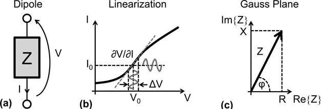
Figure 5.1 Impedance Z of a generic two-terminal element (a) whose non-linear I/V characteristic can be linearized (b) and treated as (c) a vector in the complex Gauss plane.

Impedance spectra can be displayed in two ways: in the Bode plot and in the Cole-Cole plot. As illu...