Statistical Misconceptions

Schuyler W. Huck

• Publisher: Routledge
• Year: 2008
• Print ISBN: 9780805859027
• eBook ISBN: 9781135596347
• Topic: Education
• Subtopic: Education Theory & Practice

Brief and inexpensive, this engaging book helps readers identify and then discard 52 misconceptions about data and statistical summaries. The focus is on major concepts contained in typical undergraduate and graduate courses in statistics, research methods, or quantitative analysis. Fun interactive Internet exercises that further promote undoing the misconceptions are found on the book's website.

The author's accessible discussion of each misconception has five parts:

• The Misconception - a brief description of the misunderstanding
• Evidence that the Misconception Exists – examples and claimed prevalence
• Why the Misconception is Dangerous – consequence of having the misunderstanding
• Undoing the Misconception - how to think correctly about the concept
• Internet Assignment - an interactive activity to help readers gain a firm grasp of the statistical concept and overcome the misconception.

The book's statistical misconceptions are grouped into 12 chapters that match the topics typically taught in introductory/intermediate courses. However, each of the 52 discussions is self-contained, thus allowing the misconceptions to be covered in any order without confusing the reader. Organized and presented in this manner, the book is an ideal supplement for any standard textbook.

Statistical Misconceptions is appropriate for courses taught in a variety of disciplines including psychology, medicine, education, nursing, business, and the social sciences. The book also will benefit independent researchers interested in undoing their statistical misconceptions.

1

C H A P T E R

Descriptive Statistics

There is evidence that, despite best efforts, many students and also some teachers and researchers have persistent statistical misconceptions.*

The trouble with statistics is that they are often counter-intuitive. What seems like a common sense answer to a question is often wrong.^†

1.1 Measures of Central Tendency

The Misconception

There are three different measures of central tendency: the mean, the median, and the mode.

Evidence That This Misconception Exists*

The first of the following statements comes from a recent peer-reviewed article in the medical field. The second statement comes from a book dealing with quality control. The third statement comes from an online U.S. government document.

1. The central tendency is the tendency of the observations to accumulate at a particular value or in a particular category. The three ways of describing this phenomenon are mean, median,and mode.

2. There are three measures of central tendency: mean, median, and mode.

3. There are three kinds of average: the mean, the median, and the mode.

Why This Misconception Is Dangerous

Various measures of central tendency have been invented because the proper notion of the “average” score can vary from study to study. Depending on the kind of data collected, the degree of skewness in the data, and the possible existence of outliers, it may be that the most appropriate measure of central tendency is found by doing something other than (1) dividing the sum of the scores by the number of scores (to get the mean), (2) calculating the midpoint in the distribution (to get the median), or (3) determining the most frequently observed score (to get the mode).

If you are familiar with only the arithmetic mean, the median, and the mode, you'll find yourself guilty of trying to “cram a square peg into a round hole” if a situation calls for one of the lesser known measures of central tendency. A popular little puzzle question makes this point:

If a car travels at a constant rate of 40 miles per hour between points A and B but then makes the return trip at a constant rate of 60 miles per hour, what is the car's average speed?

Here, as in certain situations involving real data, one of the lesser known averages is called for.

Undoing the Misconception

It is best to think of the various kinds of central tendency indices as falling into three categories based on the computational procedures one uses to summarize the data. One category deals with means, with techniques put into this category if scores are added together and then divided by the number of scores that are summed. The second category involves different kinds of medians, with various techniques grouped here if the goal is to find some sort of midpoint. The third category contains different kinds of modes, with these techniques focused on the frequency with which scores appear in the data.

In the first category (means), we obviously find the arithmetic mean. However, other entries in this category include the geometric mean, harmonic mean, trimmed mean, winsorized mean, midmean, and quadratic mean.*

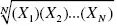
• The geometric mean is equal to

. For example, the geometric mean of 2, 3, and 36 is equal to

, which is 6.

• The harmonic mean is equal to N divided by

. For example, the harmonic mean of 2, 4, and 4 is equal to 3/[(1/2) + (1/4) + (1/4)], which is 3.

• The trimmed mean is the arithmetic average of the scores that remain after discarding the highest and lowest pth percent of the data. For example, the trimmed mean might be computed as the arithmetic mean of the middle 80% of the scores.

• The winsorized mean is the arithmetic average of all N scores after replacing the highest and lowest pth percent of the scores with the highest and lowest observed scores located on the “edges” of the middle section of scores. For example, the winsorized mean of the scores 1, 2, 4, 6, 8, and 21 might involve replacing the 1 with a 2 and the 21 with an 8, thus making the winsorized mean equal to 5.

• The midmean is the arithmetic mean of the middle 50% of the scores. For example, the midmean of the 12 scores 2, 3, 4, 6, 6, 6, 8, 8, 8, 9, 13, and 30 is 7.

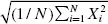
• The quadratic mean is equal to

. For example, the quadratic mean of 1, 1, 7, and 7 is 5.

In the second category (medians), we of course find the traditional median (which is equivalent to Q₂, the 50th percentile). Three other kinds of central tendency also belong in this category: midrange, midhinge, and trimean.*

• The midrange is the halfway point between the high and low scores. With 12 scores equal to 2, 3, 4, 6, 6, 6, 8, 8, 8, 9, 13, and 30, the midrange is equal to 16.

• The midhinge is the halfway point between Q₁ (the 25th percentile point) and Q₃ (the 75th percentile point). Thus, with eight scores equal to 3, 3, 5, 6, 8, 8, 10, and 14, the midhinge is equal to 6.5.

• The trimean is equal to (Q₁ + 2Q₂ + Q₃)/4, where Q₁, Q₂, and Q₃ are the lower, middle, and upper quartile points, respectively. For example, the trimean for the 12 scores 2, 3, 4, 6, 6, 6, 8, 8, 8, 9, 13, and 30 = [5 + 2(7) + 8.5]/4 = 6.875.

The third category of central tendency indices involves modes. Here, we find the traditional notion of the mode: the most frequently occurring score in the data set. In addition, three additional kinds of modes exist: minor mode, crude mode, and refined mode.

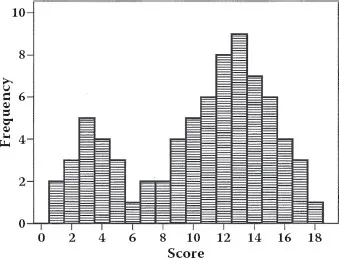
• The minor mode is the most frequently occurring score in the smaller of the 2 “humps” of a bimodal distribution. Thus, the minor mode is equal to 3 for the data displayed in Figure 1.1.1.*

• The crude mode is simply the midpoint of the modal interval in a grouped frequency distribution. For example, the crude mode for the data in Table 1.1.1 is equal to 17, the midpoint of the interval containing 10 of the 31 scores.

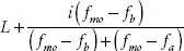
• The refined mode also deals with a grouped frequency distribution.^† The refined mode adjusts the crude mode by considering the frequencies of the intervals adjacent to the modal interval. It is computed as

where L = the lower limit of the modal interval, i = the interval width, f_mo = the frequency in the modal interval, f_b = the frequency in the interval immediately below the modal interval, and f_a = the frequency in the interval immediately above the modal interval. For the frequency distribution, the refined mode is equal to 15.5.

Internet Assignment

Would you like to see how different measures of central tendency produce radically different numerical values for the “average” score, even when they are based on the same data? Would you like to do this in a fast manner using an Internet-based, interactive Java applet that lets you control the size of each score and the number of scores in the group?

FIGURE 1.1.1 Major and minor modes in a bimodal distribution.

TABLE 1.1.1. A Frequency Distribution Summarizing 31 Scores
Interval	Frequency
35–39	2
30–34	2
25–29	3
20–24	2
15–19	10
10–14	8
5–9	3
0–4	1

If you would like to see some proof that different measures of central tendency can yield highly different results, visit this book's companion Web site (http://www.psypress.com/stati...

Table of contents

• Front Cover
• Half Title
• Title Page
• Copyright
• Dedication
• Brief Contents
• Contents
• Preface
• 1 Descriptive Statistics
• 2 Distributional Shape
• 3 Bivariate Correlation
• 4 Reliability and Validity
• 5 Probability
• 6 Sampling
• 7 Estimation
• 8 Hypothesis Testing
• 9 t-Tests Involving One or Two Means
• 10 ANOVA and ANCOVA
• 11 Practical Significance, Power, and Effect Size
• 12 Regression
• Appendix A: Citations for Material Referenced in the Preface
• Appendix B: References for Quotations Presented in the Sections Entitled “Evidence That This Misconception Exists”
• Subject Index
• Author Index