
- 232 pages
- English
- ePUB (mobile friendly)
- Available on iOS & Android
eBook - ePub
Introduction to Feedback Control Theory
About this book
There are many feedback control books out there, but none of them capture the essence of robust control as well as Introduction to Feedback Control Theory. Written by Hitay Özbay, one of the top researchers in robust control in the world, this book fills the gap between introductory feedback control texts and advanced robust control texts.
Introduction to Feedback Control Theory covers basic concepts such as dynamical systems modeling, performance objectives, the Routh-Hurwitz test, root locus, Nyquist criterion, and lead-lag controllers. It introduces more advanced topics including Kharitanov's stability test, basic loopshaping, stability robustness, sensitivity minimization, time delay systems, H-infinity control, and parameterization of all stabilizing controllers for single input single output stable plants. This range of topics gives students insight into the key issues involved in designing a controller.
Occupying and important place in the field of control theory, Introduction to Feedback Control Theory covers the basics of robust control and incorporates new techniques for time delay systems, as well as classical and modern control. Students can use this as a text for building a foundation of knowledge and as a reference for advanced information and up-to-date techniques
Trusted by 375,005 students
Access to over 1.5 million titles for a fair monthly price.
Study more efficiently using our study tools.
Information
Chapter 1
Introduction
1.1 Feedback Control Systems
Examples of feedback are found in many disciplines such as engineering, biological sciences, business, and economy. In a feedback system there is a process (a cause-effect relation) whose operation depends on one or more variables (inputs) that cause changes in some other variables. If an input variable can be manipulated, it is said to be a control input, otherwise it is considered a disturbance (or noise) input. Some of the process variables are monitored; these are the outputs. The feedback controller gathers information about the process behavior by observing the outputs, and then it generates the new control inputs in trying to make the system behave as desired. Decisions taken by the controller are crucial; in some situations they may lead to a catastrophe instead of an improvement in the system behavior. This is the main reason that feedback controller design (i.e., determining the rules for automatic decisions taken by the feedback controller) is an important topic.
A typical feedback control system consists of four subsystems: a process to be controlled, sets of sensors and actuators, and a controller, as shown in Figure 1.1. The process is the actual physical system that cannot be modified. Actuators and sensors are selected by process engineers based on physical and economical constraints (i.e., the range of signals to be measured and/or generated and accuracy versus cost of these devices). The controller is to be designed for a given plant (the overall system, which includes the process, sensors, and actuators).
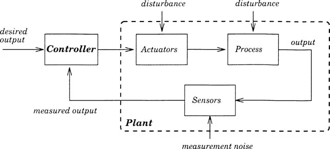
Figure 1.1: Feedback control system.
In engineering applications the controller is usually a computer, or a human operator interfacing with a computer. Biological systems can be more complex; for example, the central nervous system is a very complicated controller for the human body. Feedback control systems encountered in business and economy may involve teams of humans as main decision makers, e.g., managers, bureaucrats, and/or politicians.
A good understanding of the process behavior (i.e., the cause-effect relationship between input and output variables) is extremely helpful in designing the rules for control actions to be taken. Many engineering systems are described accurately by the physical laws of nature. So, mathematical models used in engineering applications contain relatively low levels of uncertainty, compared with mathematical models that appear in other disciplines, where input-output relationships can be much more complicated.
In this book, certain fundamental problems of feedback control theory are studied. Typical application areas in mind are in engineering. It is assumed that there is a mathematical model describing the dynamical behavior of the underlying process (modeling uncertainties will also be taken into account). Most of the discussion is restricted to single input-single output (SISO) processes. An important point to keep in mind is that success of the feedback control depends heavily on the accuracy of the process/uncertainty model, whether this model captures the reality or not. Therefore, the first step in control is to derive a simple and relatively accurate mathematical model of the underlying process. For this purpose, control engineers must communicate with process engineers who know the physics of the system to be controlled. Once a mathematical model is obtained and performance objectives are specified, control engineers use certain design techniques to synthesize a feedback controller. Of course, this controller must be tested by simulations and experiments to verify that performance objectives are met. If the achieved performance is not satisfactory, then the process model and the design goals must be reevaluated and a new controller should be designed from the new model and the new performance objectives. This iteration should continue until satisfactory results are obtained, see Figure 1.2.
Modeling is a crucial step in the controller design iterations. The result of this step is a nominal process model and an uncertainty description that represents our confidence level for the nominal model. Usually, the uncertainty magnitude can be decreased, i.e., the confidence level can be increased only by making the nominal plant model description more complicated (e.g., increasing the number of variables and equations). On the other hand, controller design and analysis for very complicated process models are very difficult. This is the basic trade-off in system modeling. A useful nominal process model should be simple enough so that the controller design is feasible. At the same time the associated uncertainty level should be low enough to allow the performance analysis (simulations and experiments) to yield acceptable results.
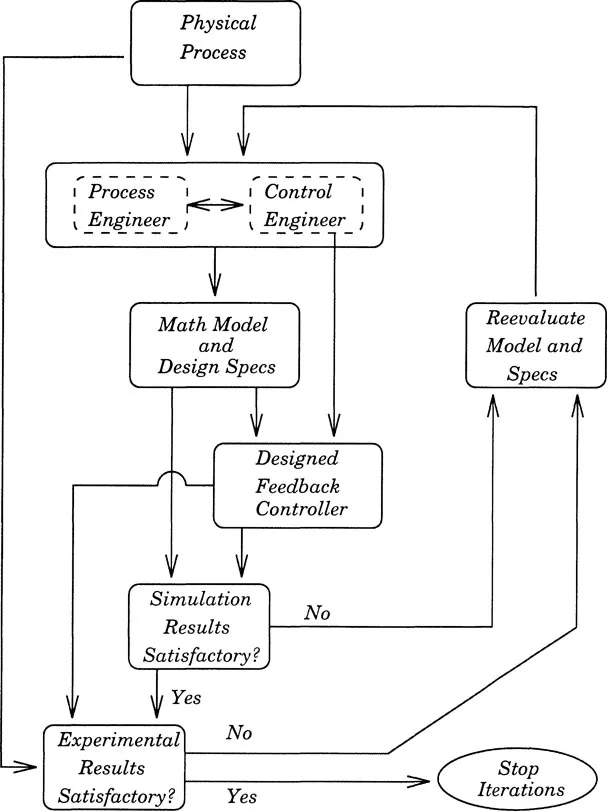
Figure 1.2: Controller design iterations.
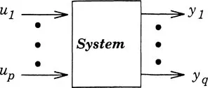
Figure 1.3: A MIMO system.
The purpose of this book is to present basic feedback controller design and analysis (performance evaluation) techniques for simple SISO process models and associated uncertainty descriptions. Examples from certain specific engineering applications will be given whenever it is necessary. Otherwise, we will just consider generic mathematical models that appear in many different application areas.
1.2 Mathematical Models
A multi-input-multi-output (MIMO) system can be represented as shown in Figure 1.3, where u1,…, up are the inputs and y1,…, yq are the outputs (for SISO systems we have p = q = 1). In this figure, the direction of the arrows indicates that the inputs are processed by the system to generate the outputs.
In general, feedback control theory deals with dynamical systems, i.e., systems with internal memory (in the sense that the output at time t = t0 depends on the inputs applied at time instants t ≤ t0). So, the plant models are usually in the form of a set of differential equations obtained from physical laws of nature. Depending on the operating conditions, input/output relation can be best described by linear or nonlinear, partial or ordinary differential equations.
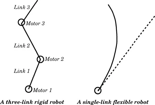
Figure 1.4: Rigid and flexible robots.
For example, consider a three-link robot as shown in Figure 1.4. This system can also be seen as a simple model of the human body. Three motors located at the joints generate torques that move the three links. Position, and/or velocity, and/or acceleration of each link can be measured by sensors (e.g., optical light with a camera, or gyroscope). Then, this information can be processed by a feedback controller to produce the rotor currents that generate the torques. The feedback loop is hence closed. For a successful controller design, we need to understand (i.e., derive mathematical equations of) how torques affect position and velocity of each link, and how current inputs to motors generate torque, as well as the sensor behavior. The relationship between torque and position/velocity can be determined by laws of physics (Newton’s law). If the links are rigid, then a set of nonlinear ordinary differential equations is obtained, see [26] for a mathematical model. If the analysis and design are restricted to small displacements around the upright equilibrium, then equations can be linearized without introducing too much error [29]. If the links are made of a flexible material (for example, in space applications the weight of the material must be minimized to reduce the payload, which forces the use of lightweight flexible materials), then we must consider bending effects of the links, see Figure 1.4. In this case, there are an infinite number of position coordinates, and partial differential equations best describe the overall system behavior [30, 46].
The robotic examples given here show that a mathematical model can be linear or nonlinear, finite dimensional (as in the rigid robot case) or infinite dimensional (as in the flexible robot case). If the parameters of the system (e.g., mass and length of the links, motor coefficients, etc.) do not change with time, then these models are time-invariant, otherwise they are time-varying.
In this book, linear time-invariant (LTI) models will be considered only. Most of the discussion will be restricted to finite dimensional models, but certain simple infinite dimensional models (in particular time delay systems) will also be discussed.
The book is organized as follows. In Chapter 2, modeling issues and sources of uncertainty are studied and the main reason to use feedback is explained. Typical performance objectives are defined in Chapter 3. In Chapter 4, basic stability tests are given. Single parameter controller design is covered in Chapter 5 by using the root locus technique. Stability robustness and stability margins are defined in Chapter 6 via Nyquist plots. Stability analysis for systems with time delays is in Chapter 7. Simple lead-lag and PID controller design methods are discussed in Chapter 8. Loopshaping ideas are introduced in Chapter 9. In Chapter 10, robust stability and performance conditions are defined and an controller design procedure is outlined. Finally, state space based controller design methods are briefly discussed and a parameterization of all stabilizing controllers is presented in Chapter 11.
Chapter 2
Modeling, Uncertainty, and Feedback
2.1 Finite Dimensional LTI System Models
Throughout the book, linear time-invariant (LTI) single input-single output (SISO) plant models...
Table of contents
- Cover
- Half Title
- Title Page
- Copyright Page
- Dedication
- Table of Contents
- 1 Introduction
- 2 Modeling, Uncertainty, and Feedback
- 3 Performance Objectives
- 4 BIBO Stability
- 5 Root Locus
- 6 Frequency Domain Analysis Techniques
- 7 Systems with Time Delays
- 8 Lead, Lag, and PID Controllers
- 9 Principles of Loopshaping
- 10 Robust Stability and Performance
- 11 Basic State Space Methods
- Bibliography
- Index
Frequently asked questions
Yes, you can cancel anytime from the Subscription tab in your account settings on the Perlego website. Your subscription will stay active until the end of your current billing period. Learn how to cancel your subscription
No, books cannot be downloaded as external files, such as PDFs, for use outside of Perlego. However, you can download books within the Perlego app for offline reading on mobile or tablet. Learn how to download books offline
Perlego offers two plans: Essential and Complete
- Essential is ideal for learners and professionals who enjoy exploring a wide range of subjects. Access the Essential Library with 800,000+ trusted titles and best-sellers across business, personal growth, and the humanities. Includes unlimited reading time and Standard Read Aloud voice.
- Complete: Perfect for advanced learners and researchers needing full, unrestricted access. Unlock 1.5M+ books across hundreds of subjects, including academic and specialized titles. The Complete Plan also includes advanced features like Premium Read Aloud and Research Assistant.
We are an online textbook subscription service, where you can get access to an entire online library for less than the price of a single book per month. With over 1.5 million books across 990+ topics, we’ve got you covered! Learn about our mission
Look out for the read-aloud symbol on your next book to see if you can listen to it. The read-aloud tool reads text aloud for you, highlighting the text as it is being read. You can pause it, speed it up and slow it down. Learn more about Read Aloud
Yes! You can use the Perlego app on both iOS and Android devices to read anytime, anywhere — even offline. Perfect for commutes or when you’re on the go.
Please note we cannot support devices running on iOS 13 and Android 7 or earlier. Learn more about using the app
Please note we cannot support devices running on iOS 13 and Android 7 or earlier. Learn more about using the app
Yes, you can access Introduction to Feedback Control Theory by Hitay Ozbay in PDF and/or ePUB format, as well as other popular books in Technology & Engineering & Differential Equations. We have over 1.5 million books available in our catalogue for you to explore.