Understanding Log-linear Analysis With Ilog

An Interactive Approach

Roger Bakeman, Byron F. Robinson

• Publisher: Psychology Press
• Year: 2013
• eBook ISBN: 9781134774692
• Edition: 1
• Topic: Psychology
• Subtopic: History & Theory in Psychology
• Index: Psychology

Whenever data are categorical and their frequencies can be arrayed in multidimensional tables, log-linear analysis is appropriate. Like analysis of variance and multiple regression for quantitative data, log-linear analysis lets users ask which main effects and interactions affect an outcome of interest. Until recently, however, log-linear analysis seemed difficult -- accessible only to the statistically motivated and savvy. Designed for students and researchers who want to know more about this extension of the two-dimensional chi-square, this book introduces basic ideas in clear and straightforward prose and applies them to a core of example studies. ILOG -- a software program that runs on IBM compatible personal computers -- is included with this volume. This interactive program lets readers work through and explore examples provided throughout the book. Because ILOG is capable of serious log-linear analyses, readers gain not only understanding, but the means to put that understanding into practice as well.

1	ANALYZING QUANTITATIVE AND QUALITATIVE SCORES: AN INTRODUCTION

In this chapter you will:

1. Review, very briefly, the multiple regression approach to analyzing quantitative data.
2. Learn in a general way when and why log-linear analyses should be used to analyze qualitative data.
3. Review, again briefly, the simple chi-square approach to analyzing qualitative data as usually presented in a basic statistics course.

For the last several decades, multiple regression or some member of its extensive family (simple correlation, t-tests, analysis of variance) has dominated data analysis in the social sciences. This understandably popular and powerful family of techniques analyzes variability in quantitative scores, and an introduction to them is provided by Understanding Social Science Statistics: A Spreadsheet Approach (Bakeman, 1992). The present volume addresses a different family of techniques, ones designed to analyze qualitative or categorical data instead. As such, although it stands alone, this book works well as a companion to Understanding Social Science Statistics.

The first chapter serves as a bridge between the two books. In the first section we review, very briefly, the multiple regression approach, stressing those ideas that appear later applied to log-linear analysis. This section should not be slighted. In it, we remind you of a number of ideas that are as important for log-linear analysis as for multiple regression. Our hope is that a thorough understanding of this first section will provide a conceptual base useful for understanding both multiple regression and log-linear approaches, and perhaps provide some integration of the two. After that, we explain in general why and when log-linear analyses should be used. Finally, we conclude this chapter with a simple chi-square example, which should serve as a review of material you probably already know but may have forgotten.

ANALYZING QUANTITATIVE SCORES: A VERY BRIEF REVIEW

As a general rule, multiple regression is appropriate whenever the factor or variable you want to account for or explain is measured on a quantitative scale (i.e., on an interval, ratio, or perhaps ordinal scale). In such cases, which are extremely frequent in the social sciences, the ability of multiple regression and its associated techniques (like analysis of variance) to estimate the proportion of variance in the dependent or criterion variable accounted for by the independent or predictor variables, and to determine whether that proportion differs significantly from zero, has proved invaluable (Bakeman, 1992; Cohen & Cohen, 1983).

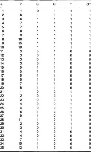
To remind you how this approach works, and to provide a bridge to the log-linear analyses with which this book is primarily concerned, imagine that you observed 20 female and 15 male infants for 5 minutes each playing with their mothers. Imagine further that you counted the number of times each infant smiled during that period and that the counts were those shown in column Y of Table 1.1. As you can see (or at least verify with your own computation), the mean number of smiles for the 20 female infants is 6.75, whereas the mean for the male infants is 5.40. Many females smiled less than many males (i.e., the distributions of the number of smiles for males and for females overlap), but overall the mean number of smiles for females is somewhat higher than the mean number for males. Still, you wonder, is this a real difference or is the difference between the means for males and females in this sample due simply to the luck of the draw, or sampling error?

What you really want to know, of course, is whether one gender smiles significantly more than the other, not just in the sample you observed but in a wider population of interest, and to answer that question you invoke the logic of hypothesis testing (see, e.g., Bakeman, 1992, chap. 2; Wickens, 1989, chap. 1). No matter how you actually recruited the infants in your study, you assume they were randomly sampled from a specified population, specifically a population in which there is no relation between gender and amount of smiling. The assumption that there is no effect of gender on the amount of smiling constitutes your null hypothesis. The null hypothesis is an important part of hypothesis testing, although as a practical matter, normally it is a hypothesis that researchers hope to refute.

TABLE 1.1
Data for the Infant Smiling Study

Note. In column heads, s represents subject number; Y represents the continuous criterion variable, number of smiles; B represents the binary criterion variable, coded 1 for five or more smiles, 0 for fewer than five smiles; G represents gender, coded 1 for female, 0 for male; T represents treatment condition, coded 1 for mobile, 0 for no mobile; and GT represents the interaction between gender and treatment.

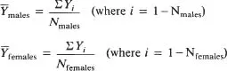
Hypothesis testing belongs to the realm of inferential statistics. But simply as a descriptive matter, and before you even invoke inferential procedures, you would probably compute the mean number of smiles for males and females in your sample, as we have already done. In general terms (letting Y-bar symbolize a mean),

Thus,

Again as a descriptive matter, you could compute the total variance in numbers of smiles for infants in the sample and the proportion of that variance accounted for by knowing an infant's gender. The total variance is

This is the average squared deviation between the observed scores and the mean for the sample (the sum of squares or SS divided by number of subjects). It represents total variability in the sample, some of which we hope to account for with independent or predictor variables. For the data in Table 1.1, total variance is 15.28, which you can (and probably should) verify. (Results of computations are usually shown in the text rounded to three significant digits; sometimes, if the first digit is 1 as here, four significant digits are displayed instead.)

The computation for total variance does not take gender into account. It pairs raw scores with the grand or overall mean. But now, imagine we define the following prediction model:

By convention, an apostrophe or prime denotes a predicted score, and so

is the predicted score for the rth infant. If X is coded 0 for males and 1 for females, then a will be the mean number of smiles for males and b will be the difference between female and male means; this follows from standard multiple regression definitions as applied to coded predictor variables (see Bakeman, 1992, chap. 11). Hence the predicted score for each male is the mean number of smiles for males (6.75 in this case), and likewise for females (5.40). In other words, if all we know is an infant's gender, the best prediction we could make for that infant's number of ...

Table of contents

• Front Cover
• Half Title
• Title Page
• Copyright
• CONTENTS
• Preface
• 1 Analyzing Quantitative and Qualitative Scores: An Introduction
• 2 Basic Statistics for Two-Dimensional Frequency Tables
• 3 Models for Two-Dimensional Frequency Tables
• 4 Fitting Models for Multidimensional Tables
• 5 ILOG Basics: Specifying a Frequency Table
• 6 Analyzing Frequency Tables with ILOG
• 7 Tallies: Enough, Too Many, None at All
• 8 Explicating Results: Percentages, Residuals, and Two-Way Tables
• References
• Glossary
• Appendix A: INSTALLING ILOG
• Appendix B: CRITICAL VALUES OF CHI SQUARE
• Author Index
• Subject Index