Multidimensional Scaling

History, Theory, and Applications

Forrest W. Young, Robert M. Hamer, Forrest W. Young, Robert M. Hamer, Robert M. Hamer, Forrest W. Young

• Publisher: Psychology Press
• Year: 2013
• eBook ISBN: 9781135059880
• Topic: Psychology
• Subtopic: History & Theory in Psychology
• Index: Psychology

This outstanding presentation of the fundamentals of multidimensional scaling illustrates the applicability of MDS to a wide variety of disciplines. The first two sections provide ground work in the history and theory of MDS. The final section applies MDS techniques to such diverse fields as physics, marketing, and political science.

I

HISTORY

Forrest W. Young

Psychometric Laboratory
University of North Carolina

1

Introduction

1.1. MDS DEFINED

Multidimensional scaling (MDS) rests on the premise that a picture is worth a thousand numbers. The term multidimensional scaling refers to a family of data analysis methods, all of which portray the data's structure in a spatial fashion easily assimilated by the relatively untrained human eye. That is, they construct a geometric representation of the data, usually in a Euclidean space of fairly low dimensionality. Some multidimensional scaling methods display the data structure in non-Euclidean spaces, and some methods provide additional information about how the structure varies over time, individuals, or experimental conditions. The essential ingredient defining all multidimensional scaling methods is the spatial representation of data structure.

Multidimensional scaling may be applied (and misapplied) to a very wide range of types of data. Essentially, any matrix of data is a candidate for analysis by some type of multidimensional scaling method, if the elements of the data matrix indicate that strength or degree of relation between the objects or events represented by the rows and columns of the data matrix. We call such data “relational” data with examples such as correlations, distances, proximities, similarities, multiple rating scales, preference matrices, etc., being well known. Multidimensional scaling methods have been designed for all types of relational data matrices, including symmetric and asymmetric matrices, rectangular and squares matrices, matrices with or without missing elements, equally and unequally replicated data matrices, two-way and multiway matrices, and other types of matrices.

1.2. POLITICAL SCIENCE EXAMPLE

The purpose of a multidimensional scaling analysis is communicated most easily by an example or two. In Table 1.1 we present a portion of a data matrix derived from voting records of U.S. Senators. Each element in this matrix represents the proportion of times a pair of Senators voted the same way on a variety of issues that came before the Senate in 1970 (the data were obtained from Hoadley, 1974). Even a very sophisticated political scientists would have to spend considerable effort to directly interpret the information as it is displayed in this table. There simply are too many numbers to make sense out of the relationships between the Senators' voting records. In Fig. 1.1 we have presented the results of a multidimensional scaling of this data matrix. When we are told that Senators who are located near each other tend to vote similarly (and conversely), then it only requires a moderate degree of familiarity with the American political scene to interpret the information displayed in the figure. The interpretation, which involves the two political parties and the degree of conservatism and liberalism of each Senator, has been added to the results of the multidimensional scaling in the form of a straight line running more or less horizontally through the figure. All Senators above this line are Republicans, and all those below are Democrats. Furthermore, those on the left are “liberals” and those on the right are “conservatives.” Note that this line, which represents the interpretation of the “Senator space” produced by the multidimensional scaling, has been added by the investigator to aid in interpreting the space. The interpretation was not part of the multidimensional scaling.

1.3. PSYCHOLOGY EXAMPLE

A second example involves a study in developmental psychology. In this study the investigator (Jacobowitz, 197S) asked children and adults to judge the similarity of various parts of the human body to each other. These judgments were used to investigate the nature of a child's conception of the body, and the way this conception changes as the child develops into an adult. The study actually involved children at three age levels (6, 8, and 10 years old), as well as college sophomores. Altogether there were 60 subjects, approximately 15 at each age level. The similarity judgments were made by the subjects in the following fashion. The experimenter selected one of the stimuli (a human body pan) and designated it as the “standard.” He then asked the subject to pick out the stimulus from those that remained (the 14 remaining stimuli are called the “comparison” stimuli), which was most similar to the standard. The experimenter then removed the picked stimulus and asked the subject to pick the stimulus from the remaining 13 comparison stimuli that

Table 1.1
Senator Voting Data

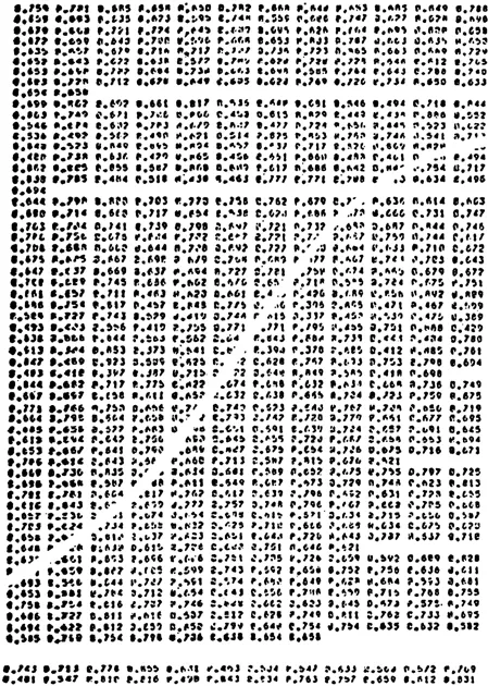
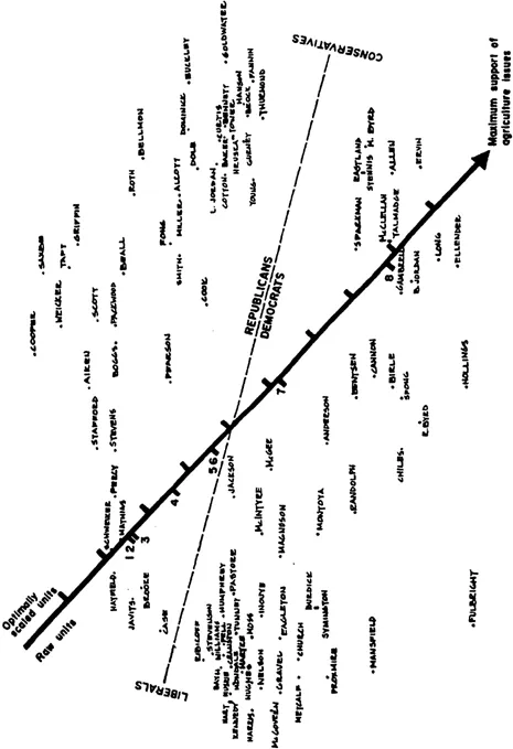
FIG. 1.1. Senator voting space.

was now most like the standard. This process was kept up until all 14 comparison stimuli had been ranked according to their similarity to the standard. The experimenter then picked out another stimulus as a standard, and repeated the task (using the same subject), getting a second rank order of 14 comparison stimuli with respect to their similarity to the second standard. This was repeated until all stimuli had served as standard (one at a time), producing 15 separate rank orders of the 14 comparison stimuli to a standard stimulus.

A portion of the data collected in this experiment is presented in Table 1.2. You will note that each row of this table contains the numbers 0–14, representing the similarity judgment. The zero, which is always on the diagonal, represents the assumption that the subject would have picked out the standard as being most similar to itself had he been able to. The 1 represents the stimulus picked first, the 2 the one picked second, etc.

Although some structure is apparent in the raw data, it becomes much clearer when we submit them to multidimensional scaling. In Fig. 1.2 we present a spatial representation of the stimuli. Again, if we know that similar stimuli are located near each other in the multidimensional space, then it is possible to develop a simple interpretation of the representation. Note that the term body is in the front part of the space, and that it is the most inclusive term being judged (i.e., all of the other terms are body parts). Note next that the terms that are the next most inclusive (arm, leg, and head) are found next as we move from the front of the space toward the back, and that the terms that are least inclusive (finger, toe, ear, etc.) are found at the back of the space. Furthermore, terms that are parts of higher level terms (e.g., toe and ankle) are directly behind the term they are included in (leg). Thus, we have the simple interpretation of the body part space as being hierarchical, keeping in mind that this interpretation is based on judgments obtained from children as well as from adults.

Of course, there is no particular reason to assume that both children and adults have the same concept of body-part structure: There might well be some sort of reliable and interesting developmental differences between these individuals. It was for this reason that the multidimensional scaling performed on these data was an individual differences multidimensional scaling, a type of multidimensional scaling that provides structural information about individuals in addition to structural information about stimuli. This additional individual differences information (which for Jacobowitz' study is really developmental differences) is displayed in Fig. 1.3. We do not explain here the precise interpretation of this figure, but you should note that the children are located in a different part of the space (on the right) than that occupied by the adults (who are on the left). Thus, we see that the multidimensional scaling has helped reveal differences between subjects. In fact, on the basis of these results, Jacobowitz concluded that the individual differences

Table 1.2
Body Part Data

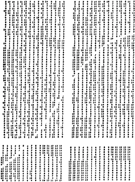
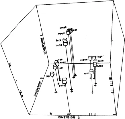
FIG. 1.2. Body-part space.

corresponded to developmental differences commensurate with theories of human development.

1.4. SOCIOLOGY EXAMPLE

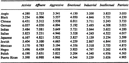
A third example comes from a sociological study of the attitudes held by American college students, about ethnic subgroups of the American society (Funk, Horowitz, Lipshitz, & Young, 1976). A portion of the data gathered in this study is presented in Table 1.3. These data represent the average, over 49 subjects, of the judged degree to which each of 13 ethnic groups could be characterized by each of 7 attributes (the 13 groups and 7 attributes are indicated in the table). In Fig. 1.4 we present the stimulus space from a multidimensional scaling of these data. (The lines have been added by the

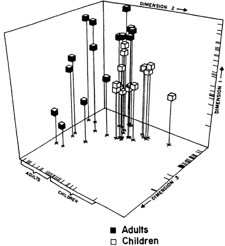
FIG. 1.3. Body-part individual difference space.

investigator to the results of the multidimensional scaling to aid in interpretation, and are not essential to the present discussion.) The basic characteristics of this space are like those of the stimulus spaces just discussed, except that there are now two sets of points embedded in the space, one for the rows of the data matrix (the ethnic group), and one for the columns of the matrix (the attributes). Thus, we have what is called a joint space because it jointly portrays the structure of the stimuli and the rating scales. (The ethnic groups are identified in the figure by the first two letters of each group's name. Black-American is indicated as.B1, for example.) Because it is still the case

TABLE 1.3
Ratings of 13 Ethnic Groups on 7 Attribute Scales

that points in the space that are close represent objects that are alike, we can discuss the similarity among the various ethnic groups, among the various adjectives, and between the groups and adjectives. However, the meaning of similarity is a little different than the foregoing. When we are discussing the structure of the groups, we have nearly the same type of interpretation as with the previous stimulus spaces. There is a slight difference, however, because the group points are located according to the judgments of the seven rating scales, not according to judged similarity. Thus, two group points that are close together tend to have the same types of ratings on the adjective scales, and two groups that are far apart tend to have very different types of ratings. It is still fair to say that the proximity of a pair of group points reflects their similarity, but we must now say that the similarity is in terms of the specific rating scales used in the experiment, not in terms of a general, nonspecific judged similarity. Thus, the space indicates that the Chinese-American group is very similar to the Japanese-American group, and that Indian-Americans are very different from Anglo-Americans, at least insofar as the rating scales used in this experiment are relevant to ethnic attitudes.

We can also make corresponding interpretations of the adjective structure. If two adjectives are located close to each other they tend to be used the same way when describing all of the groups. That is, they tend to be equally adequate or inadequate when it comes to describing each group. Thus, the multidimensional scaling indicates that the adjectives patriotic and industrious are used in the same way to describe each group, because each adjective is located in the same spot. Correspondingly, the adjectives activist and affluent are used in very different ways to describe the groups because they are located far apart in the space.

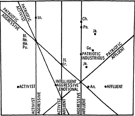
FIG. 1.4. Joint ethnic group and rating scale space.

Finally, and perhaps most interestingly, we can interpret the relationships between groups and adjectives. The interpretation is that an adjective located near a group means that the adjective is an adequate description of the group. Similarly, if the adjective and group are located far apart, then the adjective is an inadequate description. Funk et al. (1976) went on to determine the average distance from each of the adjectives to all of the ethnic groups. This procedure indicates that, on the average, affluent is closest to all of the groups and that activist is furthest. Such a finding indicates that the groups as a whole are least well described as activist and most accurately described as affluent. Of course, it is also possible to calculate the average distances from each of the ethnic groups to all of the adjectives. For example, this allows one to see that the Indian-Americans are at least well described by the adjectives used in the study, and that the Anglo-Americans are most well described. In fact, the authors concluded that this last finding, and others that may be gleaned from Fig. 1.4, reflected the operation of an experimenter bias, a possibility that usually cannot be checked in those studies of ethnic attitudes that use the standard experimental paradigms.

1.5. EXAMPLES COMPARED

It deserves emphasis that in these three examples the types of data vary widely. The first example involved a single matrix of symmetric data, far and away the most commonly used type of data for a multidimensional scaling analysis. The second example used a number of matrices, one for each subject, where each matrix was square but was asymmetric. Both of these examples involved matrices whose rows and columns represented the same set of objects (senators, in the first case, and body parts in the second). In contrast, the last example involved data that were rectangular, with the rows and columns representing different sets of objects (groups and adjectives). Note that the three examples produced different types of spatial representations, due to the different types of data being analyzed. The first one produced a Euclidean stimulus space, as did both of the other examples. However, the first two examples gave a simple space containing one set of objects, whereas the last example gave a joint space containing two sets of objects. Furthermore, the second example also produced an individual differences space, a space not provided by the other analyses. Thus, we see that the details of the geometric representation depend on the type of data being analyzed (an obvious situation, perhaps), but that all of the analyses represented the data spatially.

These three examples help illustrate the fact that multidimensional scaling is a method for analyzing data that takes an essentially incomprehensible matrix of data and represents it in a spatial fashion that is easily interpreted by the relatively untrained human eye. Multidimensional scaling extracts structure from the data and represents it in a revealing manner by relying on the fact that the user is very sophisticated when it comes to understanding the characteristics of Euclidean space. When you were told that the figures above are Euclidean models of data structure, then you knew, intuitively, how to interpret the figures. Stated most baldly, this is the reason for using Euclidean space: Through the years and years of training one has had with Euclidean space, one has learned how to “get around” in it, thus one's intuitive reactions to a Euclidean space are the “right” ones mathematically. We use the Euclidean model for the sake of convenience to the investigator, and for no other reason. We do not mean to imply that people embed hierarchical body-part structures in a Euclidean space contained in their heads, nor that the Senators carry a Senator space around in their pockets. Such notions are absurd. Rather, we use the Euclidean model as a convenient means for modeling data and nothing more.

2

History

The history of multidimensional scaling can be divided into four stages, each roughly corresponding to a decade, and each demarcated by highly innovated work.

1. The first decade was heralded by the seminal work of Torgerson (1952), who defined the multidimensional scaling problem and provided the first metric solution.

2. The second decade of work was ushered in by the path-breaking work of Shepard (1962) and Kruskal (1964) on nonmetric multidimensional scaling, and saw the highly illuminating work of Coombs (1964) on data theory.

3. The third decade opened with the trend-setting work of Carroll and Chang (1970) on individual differences multidimensional scaling, and saw the consolidation of the preceding 25 years of developments by Takane, Young, and de Leeuw (1977), and by de Leeuw and Heiser (1980).

4. The current de...

Table of contents

• Cover
• Half Title
• Full Title
• Copyright
• Dedication
• Contents
• Foreword
• Foreword
• Preface
• PART I: HISTORY
• PART II: THEORY
• PART III: APPLICATIONS
• Author Index
• Subject Index