Economic Geography

William P. Anderson

• Publisher: Routledge
• Year: 2012
• Print ISBN: 9780415701204
• eBook ISBN: 9781136293467
• Edition: 1
• Topic: Business
• Subtopic: Business General
• Index: Business

Economic geographers study and attempt to explain the spatial configuration of economic activities, including the production of goods and services, their transfer from one economic agent to another and their transformation into utility by consumers. The spatial configuration, which includes both the pattern of activities on the map and the relationships between activities occurring in different places, is the outcome of a vast number of distinct but interrelated decisions made by firms, households, governments and a variety of other private and public institutions. The goal of this book is to provide the student with a rigorous introduction to a diverse but logically consistent set of analytical models of the spatial decisions and interactions that drive the evolution of the economic landscape.

It begins by explaining fundamental concepts that are critical to all topics in economic geography: the friction of distance, agglomeration, spatial interaction, market mechanisms, natural resources and production technologies. Sections follow to cover major areas of inquiry including multiregional economies, location theory, markets for space and systems of cities. The final section synthesizes and builds on these topics to address two trends that provide particular challenges to economic geographers today: globalization and the emergence of the knowledge economy.

Part I
Fundamental concepts

1
Introduction

Economic geographers study and attempt to explain the spatial configuration of economic activities. Economic activities include all human actions that do one of three things: (1) produce goods and services, (2) transfer goods and services from one economic agent to another, and (3) transform goods and services into utility through acts of consumption. All of these activities must take place somewhere – but where? Why does a firm elect to locate its factory in a particular country, region, locality and site? Why is a retail outlet located on a main street, along a highway or in an enclosed mall? Why does a household choose to reside and consume in a particular city, suburb or rural county? These are the questions that economic geographers seek to answer.

The answers to these questions depend on the decisions of a large number of interacting economic agents – firms, households, governments, and various private and public institutions. Each agent’s choice depends on choices that have already been made, or are anticipated, by other agents. Furthermore, all decision making is influenced and constrained by the spatial distribution of environmental resources such as minerals, climate, landforms, vegetation and natural transportation corridors.

If it sounds complicated, it is. The role of the economic geographer, however, is to perceive order in all this complexity, to untangle webs of interrelated decision making and to elicit some basic principles that drive the evolution of the economic landscape. One way to do this is by building models, which attempt to abstract away from superfluous details and incidental interactions in order to focus on the main driving forces of the spatial economy. One must be careful though, complexity may in itself have implications for the evolutions of spatial patterns. Excessive abstraction may preclude an understanding of such implications.

Ultimately, the method of economic geography as it is described in this book is to use models to generate hypotheses that can then be tested against empirical observation. This, in essence, is the scientific method.¹ In order to generate hypotheses, one must ask rather specific questions. Before we can define such questions, we must ask a rather broad question that must be clearly answered before any analysis in economic geography may go forward. The question is what do we mean by space?

Discrete and continuous space

We may envision space as being either discrete or continuous. Discrete space defines a finite set of non-overlapping spatial units that make up a larger study area. They may be called regions, zones, tracts or whatever the analyst wishes. Each unit has a boundary that encloses a known area, but no further geographical detail is assigned to it. We consider the variation in income across regions, but not variations within regions. We may attempt to predict flows of people, goods or money among zones, but we are not concerned with the flows among points within a zone.

In all but a very few cases, there will be no natural division of space into units.² Thus, the first step in any analysis based in discrete space is the division of the study area by a set of boundaries which the analyst must provide. How can we avoid making boundaries that are either arbitrary or subjective? The traditional approach of geographers has been to define either of two types of regions: formal regions and functional regions. A formal region is defined as enclosing an area that is relatively homogeneous in one or a few characteristics. For example, the American Corn Belt is a formal region because it defines an area within which a relatively homogeneous type of agriculture – cultivation of corn and soybeans to feed to swine or cattle – is practiced. Anyone familiar with American agriculture has a rough idea where the Corn Belt is, but a geographer seeks to draw a boundary to determine where it is and where it isn’t. This may be done by including all areas in which the majority of farms are planted mostly in corn and soybeans. The most common formal regions are political jurisdictions such as nations, provinces, states, counties, municipalities, etc. All points within such regions are homogeneous in the sense that they are under the control of a common government.

In Figure 1.1a, we have a map of symbols representing different types of economic activities occurring at different points in space. The different symbols might represent different types of farms (grain, orchard, dairy), different classes of land users (residential, commercial, industrial) or households of different economic class (low income, middle income, high income). In Figure 1.1b, a geographer has superimposed a set of boundaries to define three regions – each with a dominant symbol – on the map.

Functional regions are defined not in terms of homogeneity but rather in terms of spatial interaction. Spatial interaction, which is one of the most critical concepts in economic geography, refers to the movement of people, goods, money or information from one place to another. A functional region is defined such that spatial interaction occurs more intensely within its borders than across them. The most common type of functional region is the metropolitan area. A metropolitan area may include a dense, low-income inner city neighborhood and a low-density, high-income suburb, along with many places that lie somewhere in between. Thus, if anything, metropolitan areas are noteworthy for their heterogeneity. Spatial interaction in the forms of commuting flows, shopping trips, deliveries of goods, phone calls and many more, however, define the metropolitan area as a functional whole. (Box 1 explains how metropolitan area boundaries used in the U.S. census are drawn based on commuting flows.)

Box 1 Defining functional regions: Metropolitan Statistical Areas in the United States

When we make reference to a city, we may be referring to two very different entities. The first is a legally defined territory within boundaries called “city limits” and under the authority of a mayor and city council. Geographers usually call this the “political city.” Referring to the definitions in chapter 1, this is an example of a formal region. The second is a geographically broader concept that includes the political city and surrounding communities that make up a politically and socially integrated urban region. Geographers refer to this as the “metropolitan area.” Since the level of integration can be measured via various forms of spatial interaction, the metropolitan area is a functional region.

Sometimes our meaning is clear from the context. If we speak about the mayor of Detroit, we are referring to the political city. But if we speak about the Detroit automotive production complex, we are referring to facilities scattered across a broad urban field and mostly outside Detroit’s city limits, so we mean the Detroit metropolitan area. We can generally make our meaning clear by referring to the “City of Detroit” and “Metro Detroit.” Also, some cities have local names to refer to the metropolitan area, such as Greater Boston, Chicagoland, the GTA (Greater Toronto Area) or the Bay Area (San Francisco, Oakland and surrounding communities.)

Economic geographers, economists, market researchers and transportation analysts generally agree that the metropolitan area is a more useful spatial definition on which to measure things like employment, production and industrial composition. Therefore, they would like to see demographic and economic data reported at the metropolitan level, rather than just for political jurisdictions. In order for statistical agencies to provide information in that form, however, they must first draw lines on the map to determine exactly which places, peoples and things are located in a particular metropolitan area and which are not.

The U.S. government has been collecting and publishing data at the metropolitan level for about 60 years. For this purpose, it has defined 366 Metropolitan Statistical Areas (MSAs) ranging in size from just under 19 million for the New York–Northern New Jersey–Long Island MSA to just over 50,000 for the Carson City, Nevada MSA. Delineation of the MSAs is a major task not only because there are so many of them but also because their boundaries need to be readjusted over time to allow for the spread of the urban field around most cities ever further into the periphery.

The U.S. Office of Management and Budget (2000) sets the rules for defining MSAs. They start from two basic geographical entities: urbanized areas and counties. An urbanized area is some geographic entity (usually a political city) defined by the U.S. Census Bureau as having an identifiable center, an overall population density above 1,000 per square mile and a population of over 50,000. Only where an urbanized area is present is an MSA defined. Counties, of which there are more than 3,000 in the U.S., are the building blocks from which MSAs are assembled. The county in which the urbanized area is located is designated as the central county. In line with our definition of a functional region, additional counties are then added to the MSA on the basis of a key measure of spatial interaction: commuting patterns. The rule is that a county is included if it is contiguous to (that means touching) the central county or any other county in the MSA and if either 25 percent of its outbound commuting trips end in the central county or 25 percent of its inbound commuting trips originate in the central county (it is usually the former). If the county has a better than 25 percent commuting link with the central counties of two different MSAs it is assigned to the one with the stronger link. Minor variations on these rules are permitted to take account of unusual local circumstances, but the idea is to keep definition as consistent as possible across all 366 MSAs. The assignment of counties to MSAs is revised after every decennial census.

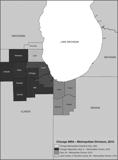
Map B1.1 shows the Chicago–Naperville–Joliet MSA. With a population of over 9 million it includes 14 counties that spill across state lines to include parts of Illinois, Indiana and Wisconsin. Cook County, which includes the City of Chicago, has more than half the total MSA population. As the map shows, when the U.S. government first defined a metropolitan area around Chicago in 1950, it included only six counties: five in Illinois and one in Indiana. Given the rule for defining the composition of MSAs, this implies that people now typically commute much longer distances to jobs in Cook County than they did in the past.

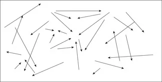
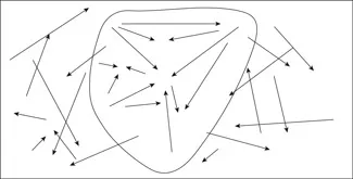
Figure 1.2a shows a set of arrows that represent daily commuting flows. The arrows begin at the residential area of commute trip origins and end at the location of the workplace destinations. In Figure 1.2b, a geographer has defined a functional region based on the commuting flows. While some flows cross the border of this region, the great majority of flows that begin within the region also end within it.

Three types of analyses can be done using discrete space. The first addresses variations in the values of one or more variables across spatial units. From a purely descriptive perspective, it might be enough to display such spatial differentiation on a map. We may go a step further and try to explain the variations by relating the value of one variable measured for each spatial unit to one or more variables measured for the same units. For example, we may be able to explain energy use per household in each U.S. state in terms of climate variables and socioeconomic variables, both of which vary across states as well.

Map B1.1 Chicago Metropolitan Statistical Area 1950, 2010

Figure 1.1a Spatial pattern of economic entities

Figure 1.1b Delineation of formal regions

Figure 1.2a Patterns of spatial interaction

Figure 1.2b Delineation of functional region

In such a ca...

Table of contents

• Cover Page
• Half Title page
• Title Page
• Copyright Page
• Dedication
• Contents
• List of illustrations
• Preface
• Acknowledgments
• Part I Fundamental concepts
• Part II The multiregional economy
• Part III Location theory
• Part IV Markets for space
• Part V Systems of cities
• Part VI Globalization and the knowledge economy
• Notes
• References
• Index