Applied Quantitative Analysis in Education and the Social Sciences

Yaacov Petscher, Christopher Schatschneider, Donald L. Compton

• Publisher: Routledge
• Year: 2013
• Print ISBN: 9780415893497
• eBook ISBN: 9781136266324
• Topic: Education
• Subtopic: Education General

To say that complex data analyses are ubiquitous in the education and social sciences might be an understatement. Funding agencies and peer-review journals alike require that researchers use the most appropriate models and methods for explaining phenomena. Univariate and multivariate data structures often require the application of more rigorous methods than basic correlational or analysis of variance models. Additionally, though a vast set of resources may exist on how to run analysis, difficulties may be encountered when explicit direction is not provided as to how one should run a model and interpret results. The mission of this book is to expose the reader to advanced quantitative methods as it pertains to individual level analysis, multilevel analysis, item-level analysis, and covariance structure analysis. Each chapter is self-contained and follows a common format so that readers can run the analysis and correctly interpret the output for reporting.

Part I

Individual-Level Analysis

1 Extending Conditional Means Modeling

An Introduction to Quantile Regression

Yaacov Petscher, Jessica A. R. Logan, and Chengfu Zhou

1.1 Why Consider Quantile Regression?

The purpose of this chapter is to introduce the reader to a special case of median regression analysis known as quantile regression. Summarizing behaviors and observations in the education and social sciences has traditionally been captured by three well-known measures of central tendency: the average of the observations, the median value, and the mode. Extensions of these descriptive measures to an inferential process are generally focused on the mean of the distribution. Traditional multiple regression analysis asks the question in the vein of, “How does X (e.g., weight) relate to Y (e.g., height)?” and implicit to this question is that the relationships among phenomena are modeled in terms of the average. Subsequently, regression may be thought of as conditional means model, in that for any given value of an independent variable, we elicit a predicted mean on the dependent variable. Since its theoretical development in 1805 by Adrien-Marie Legendre, conditional means modeling has become a universal method for model-based inferencing.

By extension, simple analysis of variance (ANOVA) models may be viewed as a special case of regression, and the more complex multilevel and structural equation models are also forms of conditional means models. Although regression is a very flexible analytic technique, it does have some weaknesses when applied to (a) non-normally distributed distributions of scores and (b) testing specific theory concerned with differential relations between constructs in a population. Related to the first point, regression is not well equipped to handle data with non-normal distributions (e.g., data with skewed or kurtotic distributions), because of its assumption that the errors are normally distributed. When this assumption is violated, the parameter estimates can be strongly biased, and the resulting p values will be unreliable (Cohen, Cohen, West, & Aiken, 2003). Within developmental and educational research, researchers are often interested in measuring skills which frequently present with non-normality based on the commonly used measures. Literacy research, for example, shows strong floor effects in the measurement of alphabet knowledge in pre-kindergarten (e.g., Paris, 2005), as well as oral reading fluency in first and second grades (e.g., Catts, Petscher, Schatschneider, Bridges, & Mendoza, 2009). Behavioral research has similarly identified floor effects when measuring dopamine activity in the brain of individuals with attention-deficit/hyperactivity disorder when differential interventions are applied (Johansen, Aase, Meyer, & Sagvolden, 2002), and researchers studying gifted populations typically observe ceiling effects in the distributions of academic achievement and aptitude (McBee, 2010).

When such distributions are encountered (for either independent or dependent variables), researchers regularly follow conventional wisdom to either transform the data to bring them closer to a normal distribution or ignore the violation of normality. Each approach may have intuitive merit; for example, when data are transformed, one is able to reflect a normal distribution of scores. Conversely, when the violation is ignored, the original metric of the score is preserved in estimating the model coefficients. In each of these conditions, limitations are presented as well. By transforming one’s data, the original metric is lost, and the interpretation of the coefficients may not have an straightforward application; yet, keeping the data in the original metric and ignoring the presence of a floor or ceiling may be misleading as the true mean relation between X and Y may be underestimated.

A second instance in which multiple regression may be insufficient to illuminate a relationship is when a theory is being tested where subgroups exist in a population on the selected outcome, and a differential relationship exists between X and Y for those different subgroups. As an example, suppose we examine the U.S. normative height (stature) growth charts for girls, ages 2 to 20 (Figure 1.1).

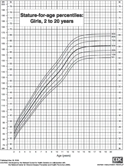
Figure 1.1 U.S. normative growth chart for height (stature) with age. From National Center for Chronic Disease Prevention and Health Promotion (2000).

The darkest black line represents the average height (y-axis) for girls at a given age (x-axis). Note that the line is very steep between ages 2 and 12 when height is still developing. For persons over age 12, height is relatively stable, and so a much weaker association between height and age is observed. Testing this theoretically heteroscedastic relationship evidenced by this illustration would be difficult using conditional means models, as the estimate of association would cloud both the lack of a relationship above age 12 and the very strong correlation up to age 12.

In response to the basic limitations of conditional means regression (i.e., non-normal distributions), a growing body of literature has begun to use quantile regression to gain more specific inferential statistics from a dataset (e.g., Catts et al., 2009). The distinguishing feature of quantile regression compared to conditional means modeling is that it allows for the estimation of relations between a dependent and independent variable at multiple locations (i.e., quantiles) of the dependent variable within a continuous distribution. That is, rather than describing the mean relations between X and Y, quantile regression estimates the relations between X and Y at multiple points in the distribution of Y. Quantile regression uses every data point when estimating a relation at a given point in the distribution of Y, asymmetrically weighting the residual errors based on the distance of each data point from the given quantile. Because of this method of estimation, quantile regression has no assumptions of the variance in the residual error terms and is robust to non-normally distributed data (Koenker, 2005).

Due to the lack of assumptions regarding the normality of the underlying distributions of scores, we believe that quantile regression lends itself well to questions in the education sciences. The goal of this chapter, therefore, is to familiarize the reader with quantile regression, its application, and the interpretation of parameters.

1.1.1 Conceptual Introduction

Regression analyses are often referred to as ordinary least squares (OLS) analyses, because they estimate a line of best fit that minimizes the squared errors between the observed and estimated values of each X value. OLS regression provides a predicted score for the outcome based on the score of the predictor(s), and is designed to estimate the relation of Y with X. Quantile regression also examines the relation of Y with X, but rather than produce coefficients which characterize the relationship in terms of the mean, as is the OLS approach, quantile regression may be viewed as a conditional median regression model. As such, the relationship between X and Y is examined conditional on the score of Y, referred to as the pth quantile. The notion of a quantile is similar to that of a percentile, whereby a score at the pth quantile reflects the place in the distribution where the proportion of the population below that value is p. For example, the .50 quantile would be akin to the 50th percentile, where 50% of the population lies below that point. In quantile regression, the .50 quantile is the median, which describes the center of the distribution in a set of data points. Quantile regression, then, predicts Y based on the score of X at multiple specific points in the distribution of Y.

As an example, suppose we were to examine the relations between children’s vocabulary scores (Y) as predicted by parental education (X). A regression of vocabulary on parental education would result in two pieces of information: (1) the intercept, which is an estimate of vocabulary score when parental education is zero, and (2) the slope coefficient, which represents the incremental change in vocabulary score (Y) for a one-unit change in parental education (X). This analytic approach answers the research question: Does parental education significantly predict children’s vocabulary scores?

Quantile regression asks a similar question as OLS, but further extends it to ask whether the relation of parental education with children’s vocabulary scores differ for children with higher or lower vocabulary scores. Entering parental education into a quantile regression equation predicting vocabulary would also result in an intercept coefficient and a slope coefficient, with the intercept representing the predicted vocabulary score when parental education is zero and the slope coefficient representing the incremental change in vocabulary score for one-unit change in parental education. However, because quantile regression estimates these relations at multiple points in the distribution of Y, the intercept and slope are uniquely estimated at several points in the distribution of vocabulary score. Because quantile regression allows the relation between X and Y to change dependent on the score of Y, it produces unique parameter estimates for each quantile it is asked to examine (e.g., the .25, .50, and .90 quantiles).

1.2 Quantile Regression Illustration in the Literature: Reading Fluency

In the previous section, we noted that OLS regression may be a limited methodological approach when the data are non-normally distributed or when the underlying theory pertains to differential effects between subgroups. In educational re...

Table of contents

• Cover
• Halftitle
• Title
• Copyright
• Dedication
• Contents
• Preface
• List of Contributors
• Part I Individual-Level Analysis
• Part II Multilevel Analysis
• Part III Item-Level Analysis
• Part IV Covariance Structure Analysis
• Index