Managing Noise and Vibration at Work

Tim South

• Publisher: Routledge
• Year: 2013
• eBook ISBN: 9781136383021
• Topic: Business
• Subtopic: Industrial Engineering
• Index: Business

New EU Physical Agents Directives on Noise and Vibration will be incorporated into UK law by February 2006. Explicit action levels for vibration will be introduced, while the action levels for noise will be drastically cut. In order to comply with these Directives, companies need to assess noise and vibration levels and provide necessary protection for their employees. They are also required to monitor and if necessary reduce noise and vibration risks.

Managing Noise and Vibration at Work introduces noise and both hand-arm and whole-body vibration by explaining what they are and how they can affect the body, drawing out the similarities and differences between the hazards. It provides clear explanations of the requirements of the EU Directives and explains how to fulfill them. Practical information on measurement, making noise and vibration assessments, and approaches to controlling risk help the reader to understand the issues of noise and vibration exposure in the workplace. The text is supported by information and diagrams of measuring equipment, advice on how to plan a survey, worked examples of necessary calculations, and charts and diagrams that can be used in place of the calculations. Suitable hearing and vibration protection is detailed. Case studies help to set the subject in context and highlight common errors and pitfalls.

The book fully covers the syllabuses of the Institute of Acoustics' certificate courses in Workplace Noise Assessment and Management of Occupational Exposure to Hand-arm Vibration. It will also be of use to those studying for the Diploma in Acoustics and Noise Control. For those studying for the NEBOSH Diploma in Health and Safety, this book satisfies modules 1E and 2E. As the Institute of Acoustics syllabuses are based on the Health and Safety Executive's guidelines, the book will also be a useful up-to-date reference for: risk managers; Health and Safety advisors and managers; occupational hygienists; environmental health officers; and HSE inspectors, especially in the Construction, Manufacturing, Agriculture and Forestry sectors.

Tim South is a Senior Lecturer in Acoustics at the School of Health and Human Sciences at Leeds Metropolitan University, and a member of the Institute of Acoustics' Education Committee. He teaches the Institute of Acoustics courses for the Certificate of Competence in Workplace Noise Assessment, the Certificate in the Management of Occupational Exposure to Hand-arm Vibration, and also the Institute's Diploma in Acoustics and Noise Control. He has extensive consultancy experience in workplace noise assessments, hand-arm vibration and whole-body vibration exposure assessments.

I

Noise

1

Noise and how it
behaves

What is noise?

Sound arises when fluctuations in air pressure give rise to pressure waves which travel through the atmosphere. As they travel they will interact in various ways with their surroundings. Noise is a word which is normally applied to unwanted sound, and the sound present in most work situations is unwanted, so we normally talk about exposure to workplace noise rather than to workplace sound.

Mathematical descriptions of how sound behaves as it interacts with solid objects can be very complicated. Fortunately it is possible to produce full descriptions of the behaviour of sound in simple, idealized situations, and to use these to build up to more realistic situations.

The simplest type of sound wave would be a pure tone – a sine wave – moving in one direction without spreading out as it moves away from the source. If you could take a snapshot of the pressure variations along the direction it was moving in, you would get a picture such as the one in Figure 1.1.

This is rather difficult to draw, so it is normally easier to show the pressure variations as a graph of pressure against distance. It should be remembered when this is done, though, that sound is a longitudinal wave. In other words the air movements as the wave progresses are backwards and forwards in the same direction as the wave as a whole is travelling. This is different from a transverse wave such as a series of ripples on a water surface, in which case the water is moving up and down while the wave travels horizontally (Figure 1.2). If you could stand at one point as the sound wave travelled towards you, and plot the pressure as a function of time, you would also get a sinusoidal shape (Figure 1.3). This is assuming you could work very fast; the pressure might be varying up and down several thousand times a second!

Even for quite loud sounds, the actual pressure change is rather small. A 1 per cent fluctuation in atmospheric pressure would be associated with an intolerably loud sound. By comparison, the atmospheric pressure can easily change by 2–3 per cent in the course of an ordinary week's weather. When we measure the magnitude of a sound wave, therefore, we concentrate on the deviations from ambient air pressure, and this deviation is normally called the sound pressure.

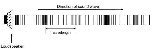
Figure 1.1 A representation of a sound wave.

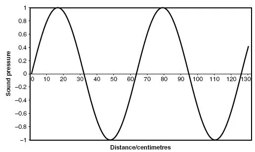
Figure 1.2 Pressure fluctuations with distance.

Pure tones, sine waves, frequency and wavelength

The sound wave described above will have a particular frequency. Essentially, the frequency of a wave is the number of complete waves which pass any particular point in the course of one second. The unit of frequency is the

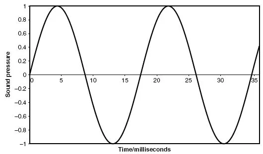
Figure 1.3 Pressure fluctuations with time.

Hertz. If the frequency is 1000 Hz (i.e. 1 kHz), then 1000 complete waves will arrive in one second. The frequency of a pure tone such as this is very closely related to its apparent pitch; a high pitched sound has a high frequency, while a low pitched tone will have a low frequency. The range of tones which are normally considered to be audible to human beings ranges from 20 to 20 000 Hz (or 20 kHz). This conceals a great deal of variation in the hearing abilities of different individuals. In particular, as human beings age they lose their ability to hear high frequencies. In any case, there is no sharp cut-off point at either end of the frequency range; it is merely necessary for sound at these extremes to be louder in order to be heard (Table 1.1).

While pure tones such as the one described above can easily be generated, most real sounds are not pure tones. Some, such as the notes produced by musical instruments, are a mixture of a relatively small number of frequencies which are related to each other (Figure 1.4). For example, a note which is based on 440 Hz may also contain components at 880, 1320, 1760 Hz and so on. Nonmusical sounds, including most of those to which people are exposed in the course of their work, do not obviously possess the property of pitch (Figure 1.5). Investigation shows that these sounds consist of a mixture of a great number of frequencies which are not related to each other in any simple mathematical way.

Table 1.1 Frequency and hearing

Frequency	Significance
20 Hz	Normally taken to be the lowest audible frequency
100 Hz	The mains hum emitted by a badly designed transformer or audio system
30–4000 Hz	Range of a piano keyboard
250–1000 Hz	Range of a female singing voice
125–6000 Hz	Range of frequencies present in speech (male voice)
200–8000 Hz	Range of frequencies present in speech (female voice)
20 000 Hz	Normally taken to be the highest audible frequency

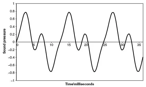
Figure 1.4 A musical note.

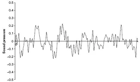
Figure 1.5 A nonmusical sound.

As well as a frequency, a sound wave at a single frequency will also have a wavelength. The wavelength is the distance between successive peaks (or between successive troughs) of a wave, and like any other length it is measured in metres. Under normal conditions, audible sounds can have wavelengths varying from a few centimetres to a few metres. At 1 kHz, for example, the wavelength will be about 34 cm. At 100 Hz, the wavelength is around 3.4 m.

The wavelength and frequency of a particular wave are related by a simple equation:

where v is the velocity with which the wave travels (this varies slightly with temperature, but is about 340 ms^–1 in air at room temperature); f is its frequency; and λ is its wavelength.

The above equation can be rewritten as

in which case it is easy to calculate the frequency corresponding to a given wavelength. Alternatively, if it is required to work out the wavelength from a knowledge of the frequency, it can be expressed as

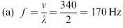
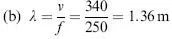
Example

(a) What is the frequency of a sound wave with a wavelength of 2 m? (b) What is the wavelength of a sound wave with a frequency of 250 Hz? Assume the speed of sound is 340 ms^–1

rms averaging

If we want to describe how loud a sound is, then we first have to produce from a waveform like the one described above, a number which describes the magnitude of the pressure fluctuations. Just averaging the deviations from normal pressure is of little use as the pressure spends as much time above the normal pressure as below it. The average would be zero. Instead, we normally get the measuring equipment to calculate the root-mean-square (rms) pressure. This is always positive and varies, as you might expect, with the loudness of a sound; loud sounds produce higher rms values than quieter ones. Other sorts of averaging could have been used, but rms averaging is widely used by electrical engineers and is useful because it relates directly to the energy content of a sound wave.

The decibel scale

A sound consists essentially of a moving series of pressure fluctuations, and the normal unit of pressure is the pascal (abbreviated to Pa). However, it is not normal to measure sound in pascals; instead the decibel (abbreviated to dB) scale is used. The decibel scale is a logarithmic one, which compresses a large range of values to a much smaller range. For example, the range of sound pressures from 0.00002 to 2.0 Pa is represented on the decibel scale by the range 0 to 100 dB. Two justifications are normally given for using a decibel scale.

1. The range of values involved in measuring the amplitude of sound is inconveniently large.

2. The human ear does not respond linearly to different sound levels and the decibel scale relates sound measurement more closely to subjective impressions of loudness.

Neither of these explanations really stands up to scrutiny. We cope with larger ranges of values when measuring other quantities (length and money are just two examples of this). It is certainly true that our ears do not respond linearly to changes in sound pressure. In other words doubling the sound pressure does not double the apparent loudness of a sound. However, they do not respond linearly to the decibel scale either, so little has been gained in this respect by using a decibel scale. Whatever the original reasons for adopting a decibel scale, it is now used universally, so there is no alternative but to do so (Table 1.2).

The use of a logarithmic scale dates from the days before electronic calculators when many calculations were carried out with the help of a book of logarithms, or ‘log’ tables. As a result, logarithms were much more familiar to anyone who needed to carry out calculations regularly. Many fewer people are nowadays familiar with them. Fortunately, with the help of a calculator, decibel calculations can be carried out without any great understanding of how logarithms work. In other fields, different logarithms – called natural logarithms and abbreviated to either log_e or ln – are used. In workplace noise calculations, all logarithms will be the more familiar system based on the number 10. They are sometimes called ‘logs to base 10’, abbreviated to log₁₀, log or simply lg.

Table 1.2 Everyday decibel levels

120 dB	Shot blasting enclosure
110 dB	Night club
100 dB	Operating position of wood planer
90 dB	Small engineering workshop
80 dB	Underground train
70 dB	Busy open-plan office
60 dB
50 dB	Private office
40 dB
30 dB	Rural location at night

The decibel scale for measuring sound levels is defined by the equation:

where L_p is the sound pressure level; p is the rms sound pressure; and p₀ is a reference pressure which has the value of 2 × 10^–5 Pa.

Example

What is the sound pressure level when the rms pressure fluctuation is 0.5 Pa?

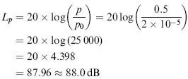
Sometimes, it is necessary to work out the rms sound pressure from a given sound pressure level. In this case, the subject of the above equation can be changed to give:

Note that whereas sound pressure level is traditionally abbreviated to SPL, and this abbreviation is still commonly seen. This book follows modern practice in using the abbreviation L_p for sound pressure level.

Addition of noise sources

Because the decibel scale is a logarithmic one, it is not possible just to add together decibel quantities. Two noise sources, each of which individually results in a sound pressure level of 70 decibels (a typical level in a busy office) will not result in anything like 140 decibels (painfully loud) when operated together. In practice, the combined level is likely to be around 73 dB, and this is because a logarithmic method must be used to combine the decibel levels. This is sometimes called decibel addition – a phrase avoided here as it might be confused with ordinary addition.

Imagine that two machines are installed in a workshop. With machine number 1 switched on and machine number 2 switched off, the measured level is L1. With machine 1 off and machine 2 on, the level is L₂. When both machines are switched on together, the combined level is given by:

Here, L_p is used to denote the combined sound levels, while the levels due to each source on its own are denoted by L₁ and L₂.

With a calculator and a little practice, calculations such as this can be carried out reasonably easily.

Example

Two machines give individual sound pressure levels at a particular workstation of 86 and 88 dB, respectively. What will be the sound pressure level when they are both switched on together?

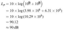
Modern calculators may give an answer in up to 10 digits. It is clearly pointless, and may be misleading, to copy all these into a report.

The convention is that the final significant figure quoted indicates the range of uncertainty of the value quoted. For example a calculator used for the above calculation offered the answer 90.12442603 dB....

Table of contents

• Front Cover
• Half Title
• Title Page
• Copyright
• Contents
• Preface
• Acknowledgements
• Part I Noise
• Part II Hand-arm Vibration
• Part III Whole Body Vibration
• Part IV Reducing Noise and Vibration Risks
• Appendix A Frequency weighting values
• Appendix B Action levels and duties
• Appendix C Glossary of symbols and abbreviations
• Appendix D Further calculation examples and answers
• Bibliography
• Index