Introduction to Digital Audio

John Watkinson

• Publisher: Routledge
• Year: 2013
• ISBN:
  9781136116933
• Edition: 2
• Topic: Technology & Engineering
• Subtopic: Acoustical Engineering
• Index: Technology & Engineering

Master the basics from first principles: the physics of sound, principles of hearing etc, then progress onward to fundamental digital principles, conversion, compression and coding and then onto transmission, digital audio workstations, DAT and optical disks. Get up to speed with how digital audio is used within DVD, Digital Audio Broadcasting, networked audio and MPEG transport streams.
All of the key technologies are here: compression, DAT, DAB, DVD, SACD, oversampling, noise shaping and error correction theories are treated in a simple yet accurate form. Thoroughly researched, totally up-to-date and technically accurate this is the only book you need on the subject.

1

Introducing digital audio

1.1 Audio as data

The most exciting aspects of digital technology are the tremendous possibilities which were not available with analog technology. Many processes which are difficult or impossible in the analog domain are straightforward in the digital domain. Once audio is in the digital domain, it becomes data, and only differs from generic data in that it needs to be reproduced with a certain timebase.

The worlds of digital audio, digital video, communication and computation are closely related, and that is where the real potential lies. The time when audio was a specialist subject which could evolve in isolation from other disciplines has gone. Audio has now become a branch of information technology (IT); a fact which is reflected in the approach of this book.

Systems and techniques developed in other industries for other purposes can be used to store, process and transmit audio, video or both at once. IT equipment is available at low cost because the volume of production is far greater than that of professional audiovisual equipment. Disk drives and memories developed for computers can be put to use in such products. Communications networks developed to handle data can happily carry audiovisual data over indefinite distances without quality loss.

As the power of processors increases, it becomes possible to perform under software control processes which previously required dedicated hardware. This allows a dramatic reduction in hardware cost. Inevitably the very nature of audiovisual equipment and the ways in which it is used is changing along with the manufacturers who supply it. The computer industry is competing with traditional manufacturers, using the economics of mass production.

Tape is a linear medium and it is necessary to wait for the tape to wind to a desired part of the recording. In contrast, the head of a hard disk drive can access any stored data in milliseconds. This is known in computers as direct access and in audio production as non-linear access. As a result the non-linear editing workstation based on hard drives has eclipsed the use of tape for editing.

Digital broadcasting uses coding techniques to eliminate the interference, fading and multipath reception problems of analog broadcasting. At the same time, more efficient use is made of available bandwidth. The hard drive-based consumer audio recorder gives the consumer more power.

Figure 1.1 Audio system of the future based on data technology.

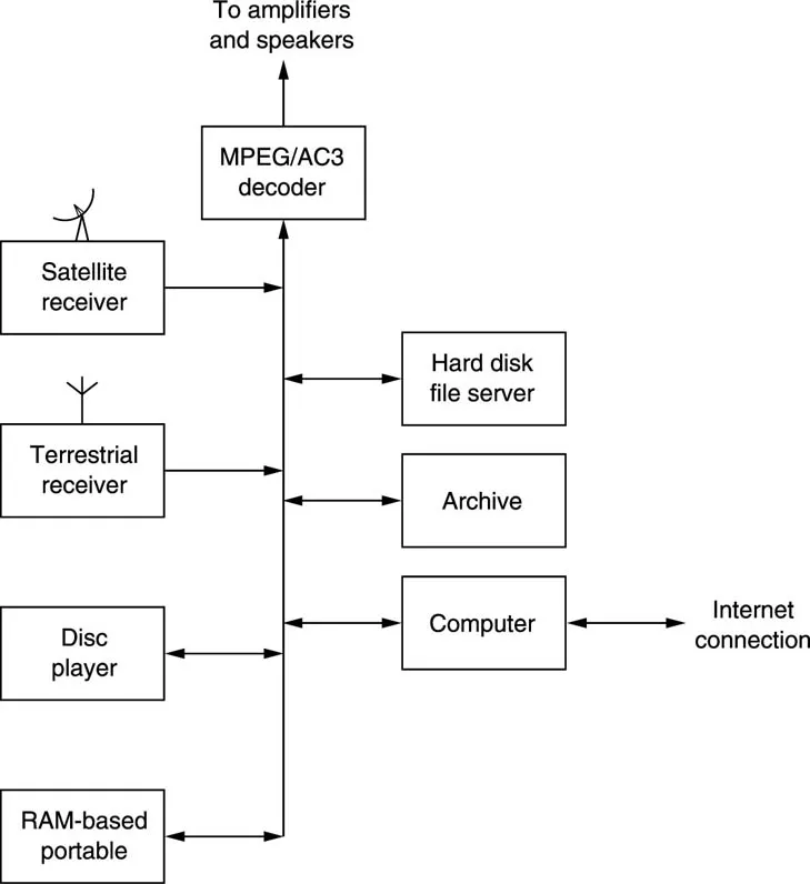
Figure 1.1 shows what the home audio system of the future may look like. MPEG-compressed signals may arrive in real time by terrestrial or satellite broadcast, via the Internet, or as the soundtrack of media such as DVD. Media such as Compact Disc supply uncompressed data for higher quality. The heart of the system is a hard drive-based server. This can be used to time shift broadcast programs, to skip commercial breaks or to assemble requested audio material transmitted in non-real time at low bit rates. If equipped with a web browser, the server may explore the web looking for material which is of the same kind the user normally wants. As the cost of storage falls, the server may download this material speculatively.

For portable use, the user may download compressed audio files into memorybased devices which act as audio players yet have no moving parts. On playback the bitstream is recovered from memory, decoded and converted typically to a signal which can drive headphones.

Ultimately digital technology will change the nature of broadcasting out of recognition. Once the viewer has non-linear storage technology and electronic program guides, the traditional broadcaster’s transmitted schedule is irrelevant. Increasingly consumers will be able to choose what is played and when, rather than the broadcaster deciding for them. The broadcasting of conventional commercials will cease to be effective when viewers have the technology to skip them. Anyone with a web site which can stream audio data can become a broadcaster.

1.2 What is an audio signal?

An analog audio signal is an electrical waveform which is a representation of the velocity of a microphone diaphragm. Such a signal is two-dimensional in that it carries a voltage changing with respect to time. In analog systems, these waveforms are conveyed by some infinite variation of a continuous parameter. In a recorder, distance along the medium is a further, continuous, analog of time. It does not matter at what point a recording is examined along its length, a value will be found for the recorded signal. That value can itself change with infinite resolution within the physical limits of the system.

Those characteristics are the main weakness of analog signals. Within the allowable bandwidth, any waveform is valid. If the speed of the medium is not constant, one valid waveform is changed into another valid waveform; a problem which cannot be detected in an analog system and which results in wow and flutter. In addition, a voltage error simply changes one valid voltage into another; noise cannot be detected in an analog signal. Noise might be suspected, but how is one to know what proportion of the received signal is noise and what is the original? If the transfer function of a system is not linear, distortion results, but the distorted waveforms are still valid; an analog system cannot detect distortion. Again distortion might be suspected, but it is impossible to tell how much of the energy at a given frequency is due to the distortion and how much was actually present in the original signal.

It is a characteristic of analog systems that degradations cannot be separated from the original signal, so nothing can be done about them. At the end of a system a signal carries the sum of all degradations introduced at each stage through which it passed. This sets a limit to the number of stages through which a signal can be passed before it is useless. Alternatively, if many stages are envisaged, each piece of equipment must be far better than necessary so that the signal is still acceptable at the end. The equipment will naturally be more expensive.

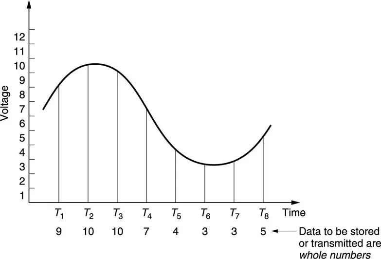
Digital audio is simply an alternative means of carrying an audio waveform. Although there are a number of ways in which this can be done, there is one system, known as pulse code modulation (PCM), which is in virtually universal use.1 Figure 1.2 shows how PCM works. Instead of being continuous, the time axis is represented in a discrete, or stepwise manner. The audio waveform is not carried by continuous representation, but by measurement at regular intervals. This process is called sampling and the frequency with which samples are taken is called the sampling rate or sampling frequency F_s. Each sample still varies infinitely as the original waveform did. To complete the conversion to PCM, each sample is then represented to finite accuracy by a discrete number in a process known as quantizing.

At the ADC (analog-to-digital convertor), every effort is made to rid the sampling clock of jitter, or time instability, so every sample is taken at an exactly even time step. Clearly, if there is any subsequent timebase error, the instants at which samples arrive will be changed and the effect can be detected. If samples arrive at some destination with an irregular timebase, the effect can be eliminated by temporarily storing the samples in a memory and reading them out using a stable, locally generated clock. This process is called timebase correction and all properly engineered digital audio systems will use it.

Figure 1.2 In pulse code modulation (PCM) the analog waveform is measured periodically at the sampling rate. The voltage (represented here by the height) of each sample is then described by a whole number. The whole numbers are stored or transmitted rather than the waveform itself.

Those who are not familiar with digital principles often worry that sampling takes away something from a signal because it appears not to be taking notice of what happened between the samples. This would be true in a system having infinite bandwidth, but no analog signal can have infinite bandwidth. All analog signal sources from microphones and so on have a resolution or frequency response limit, as indeed do devices such as loudspeakers and human hearing. When a signal has finite bandwidth, the rate at which it can change is limited, and the way in which it changes becomes predictable. When a waveform can only change between samples in one way, it is then only necessary to convey the samples and the original waveform can be unambiguously reconstructed from them. A more detailed treatment of the principle will be given in Chapter 4.

As stated, each sample is also discrete, or represented in a stepwise manner. The magnitude of the sample, which will be proportional to the voltage of the audio signal, is represented by a whole number. This process is known as quantizing and results in an approximation, but the size of the error can be controlled until it is negligible. The link between quality and sample resolution is explored in Chapter 4. The advantage of using whole numbers is that they are not prone to drift.

If a whole number can be carried from one place to another without numerical error, it has not changed at all. By describing audio waveforms numerically, the original information has been expressed in a way which is more robust.

Essentially, digital audio carries the sound numerically. Each sample is a numerical analog of the voltage at the corresponding instant in the sound.

1.3 Why binary?

Arithmetically, the binary system is the simplest numbering scheme possible.

Figure 1.3(a) shows that there are only two symbols: 1 and 0. Each symbol is a binary digit, abbreviated to bit. One bit is a datum and many bits are data. Logically, binary allows a system of thought in which statements can only be true or false.

Figure 1.3 Binary digits (a) can only have two values. At (b) are shown some everyday binary terms, whereas (c) shows some terms which cannot be expressed by a binary digit.

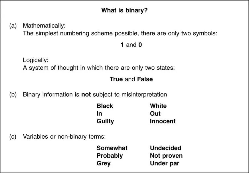
The great advantage of binary systems is that they are the most resistant to misinterpretation. In information terms they are robust. Figure 1.3(b) shows some binary terms and (c) some non-binary terms for comparison. In all real processes, the wanted information is disturbed by noise and distortion, but with only two possibilities to distinguish, binary systems have the greatest resistance to such effects.

Figure 1.4(a) shows an ideal binary electrical signal is simply two different voltages: a high voltage representing a true logic state or a binary 1 and a low voltage representing a false logic state or a binary 0. The ideal waveform is also shown at (b) after it has passed through a real system. The waveform has been considerably altered, but the binary information can be recovered by comparing the voltage with a threshold which is set half-way between the ideal levels. In this way any received voltage which is above the threshold is considered a 1 and any voltage below is considered a 0. This process is called slicing, and can reject significant amounts of unwanted noise added to the signal. The signal will be carried in a channel with finite bandwidth, and this limits the slew rate of the signal; an ideally upright edge is made to slope.

Figure 1.4 An ideal binary signal (a) has two levels. After transmission it may look like (b), but after slicing the two levels can be recovered. Noise on a sliced signal can result in jitter (c), but reclocking combined with slicing makes the final signal identical to the original as shown in (d).

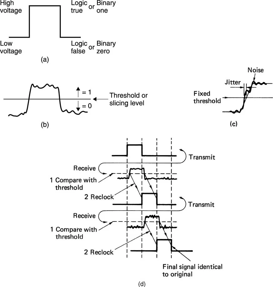
Noise added to a sloping signal (c) can change the time at which the slicer judges that the level passed through the threshold. This effect is also eliminated when the output of the slicer is reclocked. Figure 1.4(d) shows that however many stages the binary signal passes through, the information is unchanged except for a delay. Of course, an excessive noise could cause a problem. If it had sufficient level and an appropriate polarity, noise could force the signal to cross the threshold and the output of the slicer would then be incorrect. However, as binary has only two symbols, if it is known that the symbol is incorrect, it need only be set to the other state and a perfect correction has been achieved. Error correction really is as trivial as that, although determining which bit needs to be changed is somewhat harder.

Figure 1.5 shows that binary information can be represented by a wide range of real phenomena. All that is needed is t...