Deep Learning for Remote Sensing Images with Open Source Software

Rémi Cresson

• Publisher: CRC Press
• Year: 2020
• ISBN:
  9781000093612
• Edition: 1
• Topic: Technik & Maschinenbau
• Subtopic: Bauingenieurwesen

In today's world, deep learning source codes and a plethora of open access geospatial images are readily available and easily accessible. However, most people are missing the educational tools to make use of this resource. Deep Learning for Remote Sensing Images with Open Source Software is the first practical book to introduce deep learning techniques using free open source tools for processing real world remote sensing images. The approaches detailed in this book are generic and can be adapted to suit many different applications for remote sensing image processing, including landcover mapping, forestry, urban studies, disaster mapping, image restoration, etc. Written with practitioners and students in mind, this book helps link together the theory and practical use of existing tools and data to apply deep learning techniques on remote sensing images and data.

Specific Features of this Book:

• 
  
  

• The first book that explains how to apply deep learning techniques to public, free available data (Spot-7 and Sentinel-2 images, OpenStreetMap vector data), using open source software (QGIS, Orfeo ToolBox, TensorFlow)

• 
  
  

• Presents approaches suited for real world images and data targeting large scale processing and GIS applications

• 
  
  

• Introduces state of the art deep learning architecture families that can be applied to remote sensing world, mainly for landcover mapping, but also for generic approaches (e.g. image restoration)

• 
  
  

• Suited for deep learning beginners and readers with some GIS knowledge. No coding knowledge is required to learn practical skills.

• 
  
  

• Includes deep learning techniques through many step by step remote sensing data processing exercises.

Part I

Backgrounds

1

Deep learning background

In this section, we provide the essential principles of deep learning. After reading this chapter, one should have the required theoretical basis to understand what is involved in processing geospatial data in the rest of the book.

1.1 What is deep learning?

Deep learning is becoming increasingly important to solve a number of image processing tasks [1]. Among common algorithms, Convolutional Neural Network- and Recurrent Neural Network-based systems achieve state-of-the-art results on satellite and aerial imagery in many applications. For instance, synthetic aperture radar (SAR) interpretation with target recognition [2], classification of SAR time series [3], parameter inversion [4], hyperspectral image classification [5], anomaly detection [6], very-high-resolution image interpretation with scene classification [7, 8], object detection [9], image retrieval [10], and classification from time series [11]. Deep learning has addressed other issues in remote sensing, like data fusion (see [12] for a review) e.g. multimodal classification [13], pansharpening [14], and 3D reconstruction.

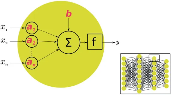
Deep learning refers to artificial neural networks with deep neuronal layers (i.e. a lot of layers). Artificial neurons and edges have parameters that adjust as learning proceeds. Inspired from biology, an artificial neuron is a mathematical function modeling a neuron. Neuron parameters (sometimes called weights) are values that are optimized during the training step. Equation 1.1 provides an example of a basic artificial neuron model. In this equation, X is the input, y the output, A the values for the gains, b is the offset value, and f is the activation function. In this minimal example, the parameters of the artificial neuron are gains and one offset value. Gains compute the scalar product with the input of the neuron, and the offset is added to the scalar product. The resulting value is passed into a non-linear function, frequently called the activation function.

y=f(AX+b)=f[∑i(ai×xi)+b]	(1.1)

Weights modify the strength of the signal at a connection. Artificial neurons may output in non-linear functions to break the linearity, for instance, to make the signal sent only if the resulting signal crosses a given threshold. Typically, artificial neurons are built in layers, as shown in figure 1.1.

FIGURE 1.1
Example of a network of artificial neurons aggregated into layers. In the artificial neuron: x_i is the input, y is the neuron output, a_i are the values for the gains, b is the offset value, and f is the activation function.

Different layers may perform different kinds of transformations on their inputs. Signals are traversing the network from the first layer (the input layer) to the last layer (the output layer), possibly after having traveled through some layers multiple times (this is the case, for instance, with layers having feedback connections). Among common networks, Convolutional Neural Networks (CNNs) achieve state-of-the-art results on images. CNNs are designed to extract features in images, enabling image recognition, object detection, and semantic segmentation. Recurrent Neural Networks (RNNs) are suited for sequential data analysis, such as speech recognition and action recognition tasks. A review of deep learning techniques applied to remote sensing can be found in [15].

In the following we will briefly present how CNN works. Basically, a CNN processes one or multiple input multidimensional arrays with a number of operations. Among these operations, we can enumerate convolution, pooling, non-linear activation functions, and transposed convolution. The input space a CNN “sees” is generally called the receptive field. Depending on the implemented operations in the net, a CNN generates an output multidimensional array with output size, dimension, and physical spacing that can be different from the input.

1.2 Convolution

Equation 1.2 shows how the result Y of a convolution with kernel K on input X is computed in dimension two (x and y are pixel coordinates). In this equation, Y and K are 2-dimensional matrices of real-valued numbers.

Y(x,y)=(X∗K)(x,y)=∑i∑jX(x−i,y−j)×K(i,j)	(1.2)

Because of the nature of the convolution, one CNN layer is composed of neurons with edges that are massively shared with the input: it can be assimilated to a small densely connected neural layer that performs the whole input locally (i.e. with connections to input restricted to a neighborhood of neurons). Generally, CNN layers are combined with non-linear activation functions and pooling operators. The convolution can be performed every Nth step in x and y dimensions: this is usually called the stride. The output of a convolution involving strides is described in equation 1.3, where s_x and s_y are the stride values in each dimension.

Y(x,y)=(X∗K)(x,y)=∑i∑jX(x×sx−i,y×sy−j)×K(i,j)	(1.3)

A convolution can be performed keeping the valid portion of the output, meaning that only the values of Y that are computed from every value of K over X are kept. In this case, the resulting output has a lower size than the input. It can also be performed over a padded input: zeros are added all around the input so that the output is computed at each location, even where the kernel doesn’t lay entirely inside the in...