Overview
This chapter serves as an introduction to the amazing and colorful world of image processing. We will start by understanding images and their various components – pixels, pixel values, and channels. We will then have a look at the commonly used color spaces – red, green, and blue (RGB) and Hue, Saturation, and Value (HSV). Next, we will look at how images are loaded and represented in OpenCV and how can they be displayed using another library called Matplotlib. Finally, we will have a look at how we can access and manipulate pixels. By the end of this chapter, you will be able to implement the concepts of color space conversion.
Introduction
Welcome to the world of images. It's interesting, it's wide, and most importantly, it's colorful. The world of artificial intelligence (AI) is impacting how we, as humans, can use the power of smart computers to perform tasks much faster, more efficiently, and with minimal effort. The idea of imparting human-like intelligence to computers (known as AI) is a really interesting concept. When the intelligence is focused on images and videos, the domain is referred to as computer vision. Similarly, natural language processing (NLP) is the AI stream where we try to understand the meaning behind the text. This technology is used by major companies for building AI-based chatbots designed to interact with customers. Both computer vision and NLP share the concepts of deep learning, where we use deep neural networks to complete tasks such as object detection, image classification, word embedding, and more. Coming back to the topic of computer vision, companies have come up with interesting use cases where AI systems have managed to change entire scenarios. Google, for example, came up with the idea of Google Goggles, which can perform several operations, such as image classification, object recognition, and more. Similarly, Tesla's self-driving cars use computer vision extensively to detect pedestrians and vehicles on the road and to detect the lane on which the car is moving.
This book will serve as a journey through the interesting components of computer vision. We will start by understanding images and then go over how they can be processed. After a couple of chapters, we will jump into detailed topics such as histograms and contours and finally go over some real-life applications of computer vision – face processing, object detection, object tracking, 3D reconstruction, and so on. This is going to be a long journey, but we will get through it together.
We love looking at high-resolution color photographs, thanks to the gamut of colors they offer. Not so long ago, however, we had photos printed only in black and white. However, those "black-and-white" photos also had some color in them, the only difference being that the colors were all shades of gray. The common thing that's there in all these components is the vision part. That's where computer vision gets its name. Computer refers to the fact that it's the computer that is processing the visual data, while vision refers to the fact that we are dealing with visual data – images and videos.
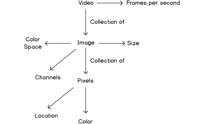
An image is made up of smaller components called pixels. A video is made up of multiple frames, each of which is nothing but an image. The following diagram gives us an idea of the various components of videos, images, and pixels:
Figure 1.1: Relationships between videos, images, and pixels
In this chapter, we will focus only on images and pixels. We will also go through an introduction to the OpenCV library, along with the functions present in the library that are commonly used for basic image processing. Before we jump into the details of images and pixels, let's get through the prerequisites, starting with NumPy arrays. The reason behind this is that images in OpenCV are nothing but NumPy arrays. Just as a quick recap, NumPy is a Python module that's used for numerical computations and is well known for its high-speed computations.
NumPy Arrays
Let's learn how to create a NumPy array in Python.
First, we need to import the NumPy module using the import numpy as np command. Here, np is used as an alias. This means that instead of writing numpy.function_name, we can use np.function_name.
We will have a look at four ways of creating a NumPy array:
- Array filled with zeros – the np.zeros command
- Array filled with ones – the np.ones command
- Array filled with random numbers – the np.random.rand command
- Array filled with values specified – the np.array command
Let's start with the np.zeros and np.ones commands. There are two important arguments for these functions:
- The shape of the array. For a 2D array, this is (number of rows, number of columns).
- The data type of the elements. By default, NumPy uses floating-point numbers for its data types. For images, we will use unsigned 8-bit integers – np.uint8. The reason behind this is that 8-bit unsigned integers have a range of 0 to 255, which is the same range that's followed for pixel values.
Let's have a look at a simple example of creating an array full of zeros. The array size should be 4x3. We can do this by using np.zeros(4,3). Similarly, if we want to create a 4x3 array full of ones, we can use np.ones(4,3).
The np.random.rand function, on the other hand, only needs the shape of the array. For a 2D array, it will be provided as np.random.rand(number_of_rows, number_of_columns).
Finally, for the np.array function, we provide the data as the first argument and the data type as the second argument.
Once you have a NumPy array, you can use npArray.shape to find out the shape of the array, where npArray is the name of the NumPy array. We can also use npArray.dtype to display the data type of the elements in the array.
Let's learn how to use these functions by completing the first exercise of this chapter.
Exercise 1.01: Creating NumPy Arrays
In this exercise, we will get some hands-on experience with the various NumPy functions that are used to create NumPy arrays and to obtain their shape. We will be using NumPy's zeros, ones, and rand functions to create the arrays. We will also have a look at their data types and shapes. Follow these steps to complete this exercise:
- Create a new notebook and name it Exercise1.01.ipynb. This is where we will write our code.
- First, import the NumPy module:
import numpy as np
- Next, let's create a 2D NumPy array with 5 rows and 6 columns, filled with zeros:
npArray = np.zeros((5,6))
- Let's print the array we just created:
print(npArray)
The output is as follows:
[[0. 0. 0. 0. 0. 0.]
[0. 0. 0. 0. 0. 0.]
[0. 0. 0. 0. 0. 0.]
[0. 0. 0. 0. 0. 0.]
[0. 0. 0. 0. 0. 0.]]
- Next, let's print the data type of the elements of the array:
print(npArray.dtype)
The output is float64.
- Finally, let's print the shape of the array:
print(npArray.shape)
The output is ...