Growth and Fluctuations 1870-1913 (Routledge Revivals)

W. Arthur Lewis

• Publisher: Routledge
• Year: 2009
• eBook ISBN: 9781135229894
• Edition: 1
• Topic: Business
• Subtopic: Business General
• Index: Business

In this title, first published in 1978, Sir Arthur Lewis considers the development of the international economy in the forty years leading up to the First World War, with the adoption of the gold standard, a rapid growth in world trade, the opening up of the continents by the railways, vast emigration from Europe, India and China, and large-scale international investment.

The book contrasts the relationship between prices, industrial fluctuations, agricultural output, and the stock of monetary gold, considering both the varying patterns of leading economies and then their net combined effect on the rest of the world. This is history which illuminates the contemporary economic climate in which it was written but also casts light upon our current economic crisis.

Chapter 1
Prospectus

SYNOPSIS: 1.00 The book is written around three interlocking themes: (a) the speed and regularity of growth of the four industrial core countries; (b) the Kondratiev swing in prices, downwards to 1895 and upwards thereafter; and (c) the differing degrees of response of countries at the periphery to the possible adoption of new technology and to opportunities to trade.

1.01 There are marked fluctuations in industrial production in the core countries. 1.02 The best known is the Juglar fluctuation, averaging about eight years. 1.03 The shorter Kitchin fluctuation is not relevant to our themes. 1.04 The Kuznets fluctuation turns on great depressions occurring about once every seventeen years. All four countries experienced such great depressions though not always simultaneously. The great depressions were associated with long swings in construction. We shall inquire whether there is a connection between great depressions and the Kondratiev swing in prices.

1.05 This long downswing followed by a long upswing is found in most price series or in their rates of change. 1.06 We shall inquire whether there was a corresponding change in the rate of growth of production. 1.07 In the downswing the terms of trade moved against farmers in both the core and the peripheral countries, stimulating political activism. The great outburst of urban radicalism at this time has also been attributed to falling prices, but the onset of the series of great depressions is a more probable cause.

1.08 The core contributed to the peripheral countries not only example but also technology, capital and migrant labour. Countries could adopt the new technology or could trade. 1.09 We shall consider why some peripheral countries responded with greater alacrity than others. 1.10 In doing so we will have to take political relationships (the colonial system) into account.

1.00 The idea of continuous economic growth from year to year is relatively new in human history; it belongs only to the period since the industrial revolution. Before that there had been long periods of economic fluctuation, including in Western Europe several low patches between 1600 and 1700. But after 1800 output per head had begun to rise steadily, and by 1900 the idea of an annual increment had joined the list of natural human rights.¹

The process of continuous growth began in England, spread during the first half of the nineteenth century to the United States, France, Belgium and Germany, in that order, and thereafter set out to conquer the whole world. For the believer in cultural diffusion, a more appropriate metaphor is that of an escalator, taking countries to ever higher levels of output per head. Countries get on to the escalator at different dates—only half a dozen before 1870, perhaps another fifteen before the First World War, another fifteen between the two world wars, and somewhat more than twenty between 1950 and 1970. The list includes peoples of all creeds, races and continents, and continues to grow.²

During the nineteenth century the escalator moved upwards at a speed of about one and a half per cent per annum (in terms of growth of output per head) but the countries on it— like the individuals on an escalator—can move faster or slower, by stepping up or down. It is also possible to fall off the escalator—to grow for a while and then to stagnate; to remain on the escalator is to have achieved the conditions for ‘sustained growth’.

Our study originates from interest in the proposition that the upward movement of those already on the escalator helps to pull more and more countries into the moving company. This proposition is not obvious, and its opposite—that it is the enrichment of the rich that impoverishes the poor is perhaps even more widely held in one form or another. Our purpose is to study the extent and mechanisms of the spread of ‘sustained growth’ during one period of time, namely the forty years before the First World War.

The theory of international trade, as the classical economists developed it, did not provide for the transmission of sustained growth (or its opposite) from one country to another, since it simply did not deal with growth: technologies are given, and neither labour nor capital migrates. The ‘dependency’ relation was introduced into economics during the inter-war period by Canadians interested in the ‘staple’ (or as we would now say, ‘exportled growth’)³ by Australians interested in the multiplier effects of an adverse balance of payments⁴ and by Englishmen blaming the great depression of the 1930s on US failure to maintain its own prosperity.⁵

The words we now use we owe to Dennis Robertson and to Raoul Prebisch. Robertson, writing in 1938, referred to international trade as ‘the engine of growth’, and Prebisch writing twelve years later referred to the relations between the industrial world and the ‘periphery’.⁶ These writers had their own definitions. In this study we shall divide the world into ‘core’ countries and the ‘periphery’.⁷ The four core countries will be Great Britain, France, Germany and the United States. The ‘engine of growth’ is the industrial sector of the core countries taken together. Our prime concern is therefore the response of the periphery to the engine of growth in the core. This atrocious mixing of metaphors may perhaps symbolise the confusion of the subject matter itself.

Core and periphery together add up to the whole world, but we are not equipped to write about the whole world, so our picture of the periphery will be general and illustrative. Furthermore, we are not writing general economic history; our focus is on rates of growth and their interactions. Even this is further restricted, since what we are seeking is the causes of growth rather than its consequences. We are taking from history only that part which seems necessary to explain core-periphery economic relations from 1870 to 1913.

What follows is thus not a systematic exposition, but a series of discussions around these three questions:

1. How fast and regular was the engine of growth (industrial production in the four core countries)?
2. What accounts for the ‘Kondratiev’ price swing, down from 1873 to 1895, and up from 1895 to 1913?
3. How does one account for the differential response of the peripheral countries?

THE ENGINE OF GROWTH AND ITS PULSATIONS

1.01 Our engine of growth is the combined industrial production of Britain, France, Germany and the United States. According to Hilgerdt⁸ this sum, by value added, was 72 per cent of world industrial production in 1913. The next two countries in size were Russia (5·5 per cent) and Italy (2·7 per cent). Our coverage seems sufficient for our purpose.

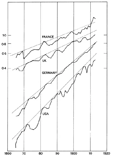
The progress of industrial production in each of these four countries is shown on semilogarithmic scale in Chart 1.1. These indexes combine manufacturing, mining and building. They are themselves controversial, and have had to be double checked before they could be used. The derivation of the British figures is explained in Appendix I, and the derivation of the others in Appendix II.

The curves are all drawn on the same scale, so their growth rates can be compared. But they are not additive, and their relative positions on the vertical scale is without significance.

Each series is shown with a line running along the top, connecting as many peaks as will fit on to a straight line. It is a peculiarity of volume series (i.e. series corrected for or not incorporating changes in price) belonging to the period 1870 to 1913 that their peaks tend to run in straight lines of this kind; this does not happen with earlier nineteenth-century series, or with series for the period between the two world wars. Even in Chart 1.1 nearly half the peaks are not strictly in line, but accuracy within one or two per cent is not to be expected of indexes of industrial production.

The line is not a trend in the statistician’s sense. It does not measure the average rate of growth of actual output, but, if anything, indicates the long-run average growth of industrial capacity.⁹ Since a straight line on a semi-logarithmic scale represents a constant annual rate of growth, the closeness of fit suggests that the fundamental determinants of industrial capacity were growing at constant rates in the four countries over these particular decades. However, we do not take this for granted; it is one of the things we want to find out.

Ultimately we shall be combining our four series to see the behaviour of the core as a whole; but since we shall not understand what happens to the whole unless we first understand what has happened to the parts, we shall first spend some time studying each of our countries individually.

First, it is obvious from the graph that the four countries grow at very different speeds. The slopes of the straight lines translate into: France 1·8 per cent per annum, UK 2·2 per cent per annum, Germany 3·9 per cent per annum, and USA 4·9 per cent per annum. Why these rates were so different is a puzzle we shall be probing.¹⁰

The graph also reveals pronounced wave-like movements in the rate of growth, which we used to call ‘cycles’. Economists have devoted an enormous literature to the study of such movements, most of it designed to show how a market economy has a built-in tendency to generate production cycles (as in the rest of economics, empirical studies are only a small fraction of the trade cycle literature). This approach is now unpopular, not because the mathematical logic is suspect, but because the models, while they explain the past satisfactorily, always fail to predict the future with reasonable accuracy. If the term ‘cycle’ is to be confined to a movement whose future can be predicted from its own past, then the movements of industrial production, though wave-like, are not cycles; and the models which can explain them backwards but not predict them forwards have to be viewed with suspicion.

Chart 1.1 Industrial Production

It does not follow that we should abandon trade cycle theory. Meteorologists can explain the path which a hurricane has taken, but cannot predict its future direction without a wide margin of error. One day they may have mastered prediction. The same may happen to economists, or it may not. To predict the course of the trade cycle requires predicting not only human behaviour, but also the physical events (such as the weather) to which human beings will have to react. So economics may always be a trade which explains the past without predicting the future. Since it is both useful and entertaining to study the past, such an exercise is not entirely without merit.

In this book we shall not be attempting to give formal or complete explanations of why fluctuations occurred. In the periphery these fluctuations came as acts of God. We shall have to know when they occurred, how intense they were, and how they affected other matters which interest us, like the volume and terms of trade, or the willingness to migrate or to invest abroad. Like the captain of a ship navigating in stormy seas we shall need to identify the waves, without needing an exhaustive theory of what causes waves.

When analysing these fluctuations economists have identified four different cycles, distinguished by length of periodicity, each of which is named after the economist who first wrote about it: the Kitchin (about three years), the Juglar (about nine years), the Kuznets (about twenty years), and the Kondratiev (about fifty years).

Since cycles are identified by dating their peaks or troughs we must first say something about this process.

First, since our engine of growth is industrial production, in this work our peaks and troughs will be those of industrial production. This yields a set of dates differing by a year or more from those yielded by other series. The traditional dating of cycles in the history books derives from financial panics—either bank failures or stock exchange collapses. This is partly because monthly and even annual data of production were scarce when trade cycle studies began in the nineteenth century, whereas financial crises are exciting and spectacular events. But it also followed from the original investigators’ belief that cycles were essentially financial phenomena, caused by fluctuations in the supply of money or credit. This approach was temporarily abandoned in the 1930s and 1940s, in favour of ‘real’ causes especially fluctuations in investment opportunities—although it is now again in favour in some circles. Some confusion results. Since some financial crises occur after the physical changes which have occasioned them, output and financial data do not always yield the same peaks, and it is somewhat jarring to be told, for example, that the crisis of 1873—one of the widest and best known—actually occurred in 1872! The idea that changes in stock exchange prices always precede real changes in the economy is a modern myth. It should be noted specifically that our peaks and troughs are not the same as those of the National Bureau of Economic Research, which constructs its reference cycles by averaging out many different financial and physical series (with the useful by-product that it can single out those which consistently lead, and use them as forecasters for the short term—say the next six months—though not for years ahead).

Secondly, a peak year has to stand out above its neighbours; but by how much? Most historians go by average levels; year 6 qualifies as a peak if it exceeds both years 5 and 7. This is not satisfactory in an economy where the labour force is growing all the time, and where investment plans presuppose built-in growth of demand. In such an economy a year which grows by less than the average will be a disappointing year; unemployment will mount, and profit expectations will be frustrated. For students of growth a peak year must exceed its predecessor by at least the normal rate of growth. As a corollary it follows that year 6 may be a peak year even if it lies below year 7. The definition of ‘normal’ will vary according to context; in the context of Chart 1.1 it is given by the slopes of the straight lines.

1.02 The standard cycle is the Juglar cycle, of about nine years’ duration. This was the first to be identified,¹¹ and since it held the field alone for about sixty years it monopolised the title of ‘the trade cycle’, and is what most people mean when they speak of ‘the cycle’. In the context of Chart 1.1 it is defined by two conditions to distinguish it from minor fluctuations:

1. Its peak is higher than all preceding points. For example, 1894 is not a Juglar peak for France. And,
2. Travelling forward from the peak, it takes more than two years to reach a year whose output exceeds that of the peak by more than two years of normal growth. (A line drawn from the peak parallel to the capacity straight line must take more than two years to touch the curve again.) Thus for France 1903 is not a Juglar peak.

On this definition the dates of the Juglar peaks are roughly: 1872/3, 1882/4, 1889/92, 1899, 1906/7 and 1912/13. It is also possible to treat 1875/6 as an extra Juglar peak for France and Germany, with some UK interest. We are not absolutely certain that 1913 would have proved to be a Juglar peak if the Great War had not erupted in 1914, but it is usually included in the list of Juglars.

One needs the double dates because the peaks do not coincide in these four countries. Naturally the countries react to each other’s fluctuations, but each has its own momentum, which yields its own timing. One must be wary of taking these figures too seriously. We are talking about differences of one per cent above or below a line, and they are not sufficiently accurate for reliable deductions in this range. Nevertheless, for what they are worth, they indicate that no single country consistently leads the others into recession. This can be seen by examining our twin peak years to see which countries turn around in the first twin year. The list is:

See Table

Each country takes its turn except Germany.

An even more remarkable sign of independence is that France, Germany and the USA all escape one or more Juglar recessions; France those of 1872 and 1907, Germany that of 1907, and the USA that of 1899. Since each of those recessions was quite severe in the other countries, the autonomous elements in each country were obviously powerful.¹²

1.03 Kitchin peaks are the Juglar peaks, plus those that were eliminated by the definition of a Juglar peak. Kitchins do not show up well in data of industrial production. They are thought to originate primarily in fluctuations in inventories and bank credit, and can be traced back to the eighteenth century, when industrial production was still small. Using again the indexes of manufacturing and mining only, one can add for the USA 1895, 1899, 1903 and 1910. US Kitchin lists usually include 1887 and 1890, which were indeed years of financial excitement, but these flurries make small dents in the industrial index. For France one can add 1872, 1889, 1894, 1903, 1907 and 1909. Our two other countries seem to have been less nervous than France and the United States. The British add only 1902, and the Germans add only 1907.

Kitchins do not help to answer any of our three basic questions, so we shall pay no more attention to them.

1.04 Kuznets cycles were identified by observing that alternate Juglar depressions in the United States were particularly severe. This was true of the years following 1872, 1892 and 1907—intervals of twenty years and fifteen years respectively. Carried forward, the series includes 1929, some twenty-two years later. Taken backwards, it is interrupted by the Civil War, which will have broken the sequence, if there was a regular sequence. Prior to that the next recession to qualify as a ‘great depression’ is that of 1837 and the early 1840s. Earlier than that it is hardly profitable to go, since industry and investment would be too small in relation to national income for their fluctuations to produce great depressions.

Here we must pause a moment to avoid semantic confusion. American writers give the title ‘great depression’ to any depression of great severity, and specifically to the five we have just enumerated: 1837, 1872, 1893, 1907 and 1929. British writers sometimes use the term for the whole of the long period of falling prices, 1873 to 1896. In this book the term is used in the American sense.

The severity of recessions is measured in various ways. A recession has two dimensions, its length and its depth. A simple way to measure its length is to count from the peak the number of years it takes to achieve two years normal growth of output, measuring normal growth as say the rate of growth between the two preceding peaks. Depth is concerned with the percentage fall from peak to trough. A recession may be shallow but long, like that starting in Britain in 1873; or deep but short, like that which succeeded it in 1883. A measure that combines length and depth is obtained by projecting a straight line forward from one Juglar peak to the next, and calculating the proportionate area between the straight line of potential capacity and the curve of actual output.

Great depressions were not confined to the Uni...

Table of contents

• Cover Page
• Title Page
• Copyright Page
• Preface
• List of Tables in the Text
• List of Tables in the Appendices
• Charts
• Chapter 1 Prospectus
• Chapter 2 The Juglar Pattern
• Chapter 3 The Kondratiev Price Swing
• Chapter 4 The Check to Real Wages
• Chapter 5 The British Climacteric
• Chapter 6 The Rate of Growth
• Chapter 7 Challenge
• Chapter 8 Response
• Chapter 9 Epilogue
• Appendix I British Statistics
• Appendix II Core Industrial Production
• Appendix III Miscellaneous Statistics
• Appendix IV World Supply of Wheat
• Notes