Signal Processing for Neuroscientists

An Introduction to the Analysis of Physiological Signals

Wim van Drongelen

• Publisher: Academic Press
• Year: 2006
• ISBN:
  9780080467757
• Topic: Biological Sciences
• Subtopic: Physiology
• Index: Biological Sciences

Signal Processing for Neuroscientists introduces analysis techniques primarily aimed at neuroscientists and biomedical engineering students with a reasonable but modest background in mathematics, physics, and computer programming. The focus of this text is on what can be considered the 'golden trio' in the signal processing field: averaging, Fourier analysis, and filtering. Techniques such as convolution, correlation, coherence, and wavelet analysis are considered in the context of time and frequency domain analysis. The whole spectrum of signal analysis is covered, ranging from data acquisition to data processing; and from the mathematical background of the analysis to the practical application of processing algorithms. Overall, the approach to the mathematics is informal with a focus on basic understanding of the methods and their interrelationships rather than detailed proofs or derivations. One of the principle goals is to provide the reader with the background required to understand the principles of commercially available analyses software, and to allow him/her to construct his/her own analysis tools in an environment such as MATLAB®.

• Multiple color illustrations are integrated in the text
• Includes an introduction to biomedical signals, noise characteristics, and recording techniques
• Basics and background for more advanced topics can be found in extensive notes and appendices
• A Companion Website hosts the MATLAB scripts and several data files: http://www.elsevierdirect.com/companion.jsp?ISBN=9780123708670

1

Introduction

1.1 OVERVIEW

Signal processing in neuroscience and neural engineering includes a wide variety of algorithms applied to measurements such as a one-dimensional time series or multidimensional data sets such as a series of images. Although analog circuitry is capable of performing many types of signal processing, the development of digital technology has greatly enhanced the access to and the application of signal processing techniques. Generally, the goal of signal processing is to enhance signal components in noisy measurements or to transform measured data sets such that new features become visible. Other specific applications include characterization of a system by its input-output relationships, data compression, or prediction of future values of the signal.

This text introduces the whole spectrum of signal analysis: from data acquisition (Chapter 2) to data processing, and from the mathematical background of the analysis to the implementation and application of processing algorithms. Overall, our approach to the mathematics will be informal, and we will therefore focus on a basic understanding of the methods and their interrelationships rather than detailed proofs or derivations. Generally, we will take an optimistic approach, assuming implicitly that our functions or signal epochs are linear, stationary, show finite energy, have existing integrals and derivatives, and so on.

Noise plays an important role in signal processing in general; therefore, we will discuss some of its major properties (Chapter 3). The core of this text focuses on what can be considered the “golden trio” in the signal processing field:

1. Averaging (Chapter 4)

2. Fourier analysis (Chapters 5Chapter 6Chapter 7)

3. Filtering (Chapters 10Chapter 11Chapter 12Chapter 13)

Most current techniques in signal processing have been developed with linear time invariant (LTI) systems as the underlying signal generator or analysis module (Chapters 8 and 9). Because we are primarily interested in the nervous system, which is often more complicated than an LTI system, we will extend the basic topics with an introduction into the analysis of time series of neuronal activity (spike trains, Chapter 14), analysis of nonstationary behavior (wavelet analysis, Chapters 15 and 16), and finally on the characterization of time series originating from nonlinear systems (Chapter 17).

1.2 BIOMEDICAL SIGNALS

Due to the development of a vast array of electronic measurement equipment, a rich variety of biomedical signals exist, ranging from measurements of molecular activity in cell membranes to recordings of animal behavior. The first link in the biomedical measurement chain is typically a transducer or sensor, which measures signals (such as a heart valve sound, blood pressure, or X-ray absorption) and makes these signals available in an electronic format. Biopotentials represent a large subset of such biomedical signals that can be directly measured electrically using an electrode pair. Some such electrical signals occur “spontaneously” (e.g., the electroencephalogram, EEG); others can be observed upon stimulation (e.g., evoked potentials, EPs).

1.3 BIOPOTENTIALS

Biopotentials originate within biological tissue as potential differences that occur between compartments. Generally the compartments are separated by a (bio)membrane that maintains concentration gradients of certain ions via an active mechanism (e.g., the Na⁺/K⁺ pump). Hodgkin and Huxley (1952) were the first to model a biopotential (the action potential in the squid giant axon) with an electronic equivalent. A combination of ordinary differential equations (ODEs) and a model describing the nonlinear behavior of ionic conductances in the axonal membrane generated an almost perfect description of their measurements. The physical laws used to derive the base ODE for the equivalent circuit are Nernst, Kirchhoff, and Ohm’s laws (Appendix 1.1). An example of how to derive the differential equation for a single ion channel in the membrane model is given in Chapter 8, Figure 8.2.

1.4 EXAMPLES OF BIOMEDICAL SIGNALS

1.4.1 EEG/ECoG and Evoked Potentials (EPs)

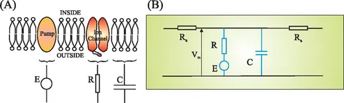
Figure 1.1 The origin of biopotentials. Simplified representation of the model described by Hodgkin and Huxley (1952). (A) The membrane consists of a double layer of phospholipids in which different structures are embedded. The ion pumps maintain gradient differences for certain ion species, causing a potential difference (E). The elements of the biological membrane can be represented by passive electrical elements: a capacitor (C) for the phospholipid bilayer and a resistor (R) for the ion channels. (B) In this way, a segment of membrane can be modeled by a circuit including these elements coupled to other contiguous compartments ...