Magnetic Resonance Spectroscopy

Tools for Neuroscience Research and Emerging Clinical Applications

Charlotte Stagg, Douglas L. Rothman

• Publisher: Academic Press
• Year: 2013
• Print ISBN: 9780124016880
• eBook ISBN: 9780124016972
• Topic: Medicine
• Subtopic: Neurology

Magnetic Resonance Spectroscopy: Tools for Neuroscience Research and Emerging Clinical Applications is the first comprehensive book for non-physicists that addresses the emerging and exciting technique of magnetic resonance spectroscopy. Divided into three sections, this book provides coverage of the key areas of concern for researchers. The first, on how MRS is acquired, provides a comprehensive overview of the techniques, analysis, and pitfalls encountered in MRS; the second, on what can be seen by MRS, provides essential background physiology and biochemistry on the major metabolites studied; the final sections, on why MRS is used, constitutes a detailed guide to the major clinical and scientific uses of MRS, the current state of teh art, and recent innovations.Magnetic Resonance Spectroscopy will become the essential guide for people new to the technique and give those more familiar with MRS a new perspective.- Chapters written by world-leading experts in the field- Fully illustrated- Covers both proton and non-proton MRS- Includes the background to novel MRS imaging approaches

Section 1

Technical Aspects—How MRS is Acquired

Outline

Chapter 1.1 Basis of Magnetic Resonance

Chapter 1.2 Localized Single-Voxel Magnetic Resonance Spectroscopy, Water Suppression, and Novel Approaches for Ultrashort Echo-Time Measurements

Chapter 1.3 Technical Considerations for Multivoxel Approaches and Magnetic Resonance Spectroscopic Imaging

Chapter 1.4 Spectral Editing and 2D NMR

Chapter 1.5 Spectral Quantification and Pitfalls in Interpreting Magnetic Resonance Spectroscopic Data

Chapter 1.1

Basis of Magnetic Resonance

Christoph Juchem^1,2 and Douglas L. Rothman¹, ¹Department of Diagnostic Radiology, ²Department of Neurology, Yale School of Medicine, Massachussetts, USA

Magnetic resonance spectroscopy (MRS) allows the detection and quantification of chemical compounds from localized portions of the living tissue, e.g., the brain, in a noninvasive fashion. The goal of this chapter is to provide an introduction to and summarize commonly applied in vivo MRS methods. The descriptions in this chapter will be kept at a relatively introductory level focusing on the basic MR physics and engineering principles involved. More information on the experimental implementation and applications of these methods are provided in subsequent chapters of this book.

Keywords

MR physics; MRS; quantitation; spectroscopy

Introduction

Magnetic resonance spectroscopy (MRS) allows the detection and quantification of chemical compounds from localized portions of the living tissue, e.g., the brain, in a noninvasive fashion. It thereby provides a powerful tool to assess key aspects of brain metabolism and function. In the clinics, the repertoire of measurable compounds along with the quantitative character of the derived information makes MRS a versatile tool for the identification of clinical conditions, for longitudinal patient monitoring and for treatment control. The goal of this chapter is to summarize the basic concepts of commonly applied in vivo MRS methods. These concepts will be developed more in subsequent chapters as well as more advanced MRS methods such as spectroscopic imaging and J-editing, and measurement of specific chemicals and metabolic pathways. The descriptions in this chapter will be kept at a relatively basic level. For a more advanced but still very accessible treatment of basic MRS spin physics as well as MRS methodology we recommend de Graaf (2008).

In Vivo Spectroscopy

Atomic nuclei with a magnetic moment (or “spin”) can exhibit resonance behavior in a magnetic field. This magnetic resonance effect is governed by the Larmor equation as a simple linear relationship between the magnetic field B perceived by the nucleus and the resultant resonance frequency ω.

(1)

The relative scaling γ, the so-called gyromagnetic ratio, is a nucleus-specific constant. The hydrogen nucleus ¹H (i.e., a proton) is the prime example for an MR-sensitive isotope as ¹H resonance signals from hydrogen nuclei bound in tissue water provide the basis for MR imaging (MRI) of the human body. Nuclear spins can be thought of as microscopic magnets. When placed in a magnetic field these magnetic moments become polarized, and are either parallel or antiparallel to the field. The spins that are polarized parallel to the field are in a lower energy state, so slightly more are present in this alignment than antiparallel to the field. When radiofrequency (RF) energy is applied to spins in a magnet at the Larmor frequency, the spins will absorb energy and undergo a transition from the antiparallel to the parallel state as with optical and other forms of resonance spectroscopy. MRS, however, differs in that in the process of absorption the spins will become polarized with the RF field such that when the RF field is shut off the spins will effectively rotate along the axis of the magnet (by convention the z-axis in MRS). This phenomenon creates a rotating magnetic field at the Larmor frequency. When an RF receiver coil is used the rotating magnetization induces an oscillating voltage by induction, which is then detected by the MR spectrometer (which is essentially a large RF transmitter and receiver). At field strengths available for clinical MRS the Larmor frequency will vary from ~60 to 300 MHz corresponding to magnet field strengths of 1.5 and 7.0 T, respectively. The low resonance frequency (6 to 7 orders of magnitude lower than optical resonances) is disadvantageous from a sensitivity standpoint, because the energy per absorption or emission is proportional to frequency. However, unlike optical spectroscopy or imaging, the human body is relatively transparent to RF at the MHz range and therefore is completely accessible to measurement by MRS.

When a human subject is placed in the scanner of a given field strength, one could assume that all of the body’s ¹H nuclei exhibit the same resonance frequency. In reality, however, minute frequency variations are observed depending on the molecular structure the atomic nucleus is embedded in. The field variations to cause these frequency shifts are based on two different effects. The electronic, i.e., the chemical, environment around the atomic nucleus at hand results in a so-called “chemical shift” and the correlation of different nuclei of the same molecule mediated through their binding electrons is referred to as dipolar or J-coupling. Chemical shift and J-coupling critically rely on the molecules’ chemical and geometric composition. As such, their measurement provides a wealth of intramolecular, microscopic information from a relatively simple, “macroscopic” MRS experiment. Notably, chemical shift and J-coupling are the basis for the key role MRS is playing in structural and analytical chemistry. Although chemical shift and J-coupling were discovered in the 1950s, it was not until 20 years later that MRS was applied to identify and quantify biochemicals in living cells (Shulman et al., 1979) and eventually in vivo (Ackerman et al., 1980). With this paradigm shift, the goal was no longer to study the physicochemical properties of substances, but to use the knowledge on the substance-specific spectroscopic patterns, i.e., their spectroscopic fingerprint, to separate and quantify these substances in vivo to infer the concentrations of metabolites and the fluxes of metabolic pathways.

MRS allows the noninvasive quantification of neurochemicals that contain MR-sensitive isotopes (e.g., ¹H). Hydrogen is prevalent in most metabolites of the human brain and the ¹H nucleus is the most relevant isotope for in vivo MRS. The gyromagnetic ratio of ¹H is highest for all stable isotopes; therefore, its sensitivity in MR experiments is higher than for any other nucleus. Furthermore, the natural abundance of the ¹H nucleus is almost 100%. The first in vivo MRS measurements of the living brain were in 1982 on a small-bore high-field MR system (Behar et al., 1983). With the subsequent rapid development of large-bore high-field magnets and volume localization by the mid-1980s, the first ¹H MR spectra of human brain were obtained (Bottomley et al., 1983; Frahm et al., 1989) and today ¹H MR spectra can be somewhat routinely obtained on all clinical MRI systems of 1.5 T and higher in field strength.

Although a series of brain metabolites can be identified with ¹H MRS (Govindaraju et al., 2000), the number of substances that are assessable under in vivo conditions does not exceed 15–20 (Mekle et al., 2009; Tkac et al., 2009; Emir et al., 2011a) and is typically well below. Further MR-visible isotopes with biochemical relevance have been shown to provide valuable information on tissue physiology and biochemistry. Phosphorus (³¹P) MRS, for instance, allows the quantification of key components of the tissues’ energy metabolism (ATP, ADP, and phosphocreatine) and to study, for example, bioenergetic deficits in response to disease (Befroy & Shulman, 2011). MRS employing the ¹³C isotope enables the study of Krebs (TCA) cycle intermediates, and the predictable transfer of infused ¹³C-label between specific positions of the carbon chains of these intermediates stands out by providing turnover rates and metabolic fluxes (Rothman et al., 2011). Today’s clinical MRS, however, mostly relies on ¹H whereas other nuclei are predominantly used in basic and preclinical research. The need for nonstandard hardware and specialized MRS methods for non-¹H MRS might be reasons why these applications have yet to prevail in clinical practice. This chapter therefore focuses on the basic principles of ¹H MRS, although where appropriate extensions to other nuclei will be discussed (for more detail on this topic see Chapters 4.1–4.3.).

MRS Methods

Basics of MRS

The goal of in vivo ¹H MRS is to quantify biochemical substances in a noninvasive fashion. In general, the signal amplitudes of an MRS acquisition and the resultant peaks in the reconstructed spectrum directly scale with the number of resonating nuclei and the substance amount seen by the MRS experiment. As such, spectral peaks and patterns provide a direct measure for the concentration of the metabolite at hand. Water is by far the most prevalent ¹H-containing compound in human tissue; therefore it contributes the largest part of the MR signal (Fig. 1.1.1A). Since the water concentration itself is of little clinical relevance, its signal is typically minimized in MRS experiments to better reveal the metabolites of interest (Fig. 1.1.1B). A prominent limitation of ¹H MRS of brain metabolites is the small frequency spread between spectral peaks. This limited spectral dispersion leads to severe spectral overlap of the observed patterns and poses a significant challenge for the identification and separation of the individual compounds. Notably, the problem of spectral overlap is further complicated in vivo by limited magnetic field homogeneity and the resultant broadening of spectral lines. The strongest limitation for the quantification of tissue metabolites, however, arises from the inherently poor sensitivity of MR methods. Metabolite concentrations in the millimolar range are therefore necessary with ¹H MRS to achieve signal amplitudes that sufficiently exceed the inevitable measurement noise. Moreover, adequate signal-to-noise ratio (SNR) is particularly relevant when partially overlapping spectral structures are to be disentangled, as is typically the case for ¹H MRS.

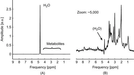
Figure 1.1.1 The role of water suppression for in vivo ¹H MRS of the human brain. (A) The water content in human brain tissue largely exceeds the concentrations of other observable substances and therefore dominates the appearance of the spectrum. (B) Suppression of the water signal allows an unobstructed vie...

Table of contents

• Cover image
• Title page
• Table of Contents
• Copyright
• Acknowledgements
• Contributors
• Introduction
• Section 1: Technical Aspects—How MRS is Acquired
• Section 2: Biochemistry — What Underlies the Signal?
• Section 3: Applications of Proton-MRS
• Section 4: Applications of Non-Proton MRS
• Index