Quantifying Life

A Symbiosis of Computation, Mathematics, and Biology

Dmitry A. Kondrashov

• Publisher: University of Chicago Press
• Year: 2016
• ISBN:
  9780226371931
• Topic: Biological Sciences
• Subtopic: Science General
• Index: Biological Sciences

Since the time of Isaac Newton, physicists have used mathematics to describe the behavior of matter of all sizes, from subatomic particles to galaxies. In the past three decades, as advances in molecular biology have produced an avalanche of data, computational and mathematical techniques have also become necessary tools in the arsenal of biologists. But while quantitative approaches are now providing fundamental insights into biological systems, the college curriculum for biologists has not caught up, and most biology majors are never exposed to the computational and probabilistic mathematical approaches that dominate in biological research.With Quantifying Life, Dmitry A. Kondrashov offers an accessible introduction to the breadth of mathematical modeling used in biology today. Assuming only a foundation in high school mathematics, Quantifying Life takes an innovative computational approach to developing mathematical skills and intuition. Through lessons illustrated with copious examples, mathematical and programming exercises, literature discussion questions, and computational projects of various degrees of difficulty, students build and analyze models based on current research papers and learn to implement them in the R programming language. This interplay of mathematical ideas, systematically developed programming skills, and a broad selection of biological research topics makes Quantifying Life an invaluable guide for seasoned life scientists and the next generation of biologists alike.

Part IV

Variables that change with time

Chapter 14

Linear difference equations

We’re captive on the carousel of time

We can’t return we can only look behind

From where we came

And go round and round and round

In the circle game

—Joni Mitchell, The Circle Game

All living things change over time, and this evolution can be quantitatively measured and analyzed. Mathematics makes use of equations to define models that change with time, known as dynamical systems. This part discusses how to construct models that describe the time-dependent behavior of some measurable quantity in life sciences. Numerous fields of biology use such models, and in particular, we will consider changes in population size, the progress of biochemical reactions, the spread of infectious disease, and the spikes of membrane potentials in neurons as some of the main examples of biological dynamical systems.

Many processes in living things happen regularly, repeating with a fairly constant time period. One common example is the reproductive cycle in species that reproduce periodically, whether once a year, or once an hour, like certain bacteria that divide at a relatively constant rate under favorable conditions. Other periodic phenomena include circadian (daily) cycles in physiology, contractions of the heart muscle, and waves of neural activity. For these processes theoretical biologists use models with discrete time, in which the time variable is restricted to the integers. For instance, it is natural to count the generations in whole numbers when modeling population growth.

This chapter is devoted to analyzing dynamical systems in which time is measured in discrete steps. In this chapter you will learn to do the following:

1. write down discrete-time (difference) equations based on stated assumptions,

2. find analytic solutions of linear difference equations,

3. define functions in R, and

4. compute numerical solutions of difference equations.

14.1 Discrete-time population models

Let us construct our first models of biological systems. We start by considering a population of some species, with the goal of tracking its growth or decay over time. The variable of interest is the number of individuals in the population, which we call N. This is called the dependent variable, since its value changes depending on time; it would make no sense to say that time changes depending on the population size. Throughout the study of dynamical systems, we will denote the independent variable of time by t. To denote the population size at time t we can write N(t) but sometimes use N_t.

14.1.1 static population

To describe the dynamics, we need to write down a rule for how the population changes. Consider the simplest case, in which the population stays the same for all time. (Maybe it is a pile of rocks?) Then the following equation describes this situation:

This equation mandates that the population at the next time step be the same as at the present time t. This type of equation is generally called a difference equation, because it can be written as a difference between the values at the two different times:

This version of the model illustrates that a difference equation at its core describes the increments of N from one time step to the next. In this case, the increments are always 0, which makes it plain that the population does not change from one time step to the next.

14.1.2 exponential population growth

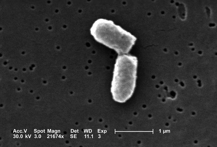
Let us consider a more interesting situation: a colony of dividing bacteria, such as Escherichia coli, shown in Figure 14.1. Assume that each bacterial cell divides and produces two daughter cells at fixed intervals of time, and let us further suppose that bacteria never die. Essentially, we are assuming a population of immortal bacteria with clocks. This means that after each cell division, the population size doubles. As before, we denote the number of cells in each generation by N(t) and obtain the equation describing each successive generation:

It can also be written in the difference form:

The increment in population size is determined by the current population size, so the population in this model is forever growing. This type of behavior is termed exponential growth, which we investigate further in section 14.2.

14.1.3 example with birth and death

Suppose that a type of fish lives to reproduce only once after a period of maturation, after which the adults die. In this simple scenario, half the population is female; a female always lays 1000 eggs; and of those, 1% survive to maturity and reproduce. Let us set up the model for the population growth of this idealized fish population. The general idea, as before, is to relate the population size at the next time step N(t + 1) to the population at the present time N(t).

Figure 14.1: Scanning electron micrograph of a dividing Escherichia coli bacteria. Image by Evangeline Sowers and Janice Haney Carr (CDC) in public domain via Wikimedia Commons.

Let us tabulate both the increases and the decreases in the population size. We have N(t) fish at the present time, but we know they all die after reproducing, ...