Elements of Acoustic Phonetics

Peter Ladefoged

• Publisher: University of Chicago Press
• Year: 2017
• ISBN:
  9780226191010
• Topic: Langues et linguistique
• Subtopic: Linguistique

This revised and expanded edition of a classic textbook provides a concise introduction to basic concepts of acoustics and digital speech processing that are important to linguists, phoneticians, and speech scientists. The second edition includes four new chapters that cover new experimental techniques in acoustic phonetics made possible by the use of computers. Assuming no background in physics or mathematics, Ladefoged explains concepts that must be understood in using modern laboratory techniques for acoustic analysis, including resonances of the vocal tract and the relation of formants to different cavities; digital speech processing and computer storage of sound waves; and Fourier analysis and Linear Predictive Coding, the equations used most frequently in the analysis of speech sounds. Incorporating recent developments in our knowledge of the nature of speech, Ladefoged also updates the original edition's discussion of the basic properties of sound waves; variations in loudness, pitch, and quality of speech sounds; wave analysis; and the hearing and production of speech.Like its predecessor, this edition of Elements of Acoustic Phonetics will serve as an invaluable textbook and reference for students and practitioners of linguistics and speech science, and for anyone who wants to understand the physics of speech.

CHAPTER ELEVEN

Digital Filters and LPC Analysis

The Fourier transform is not the only way of determining the spectrum of a sound. A technique much in use in phonetic analysis involves determining what are called the Linear Predictor Coefficients of a sound wave. This procedure, known as LPC analysis, is a little more complex than Fourier analysis by a Discrete Fourier Transform (DFT), described in the previous chapter. However, it is possible to provide a simple overview of the underlying mathematical principles that assumes nothing about matrix algebra or complex numbers. But, be warned, it will require patient working through some cumbersome elementary equations.

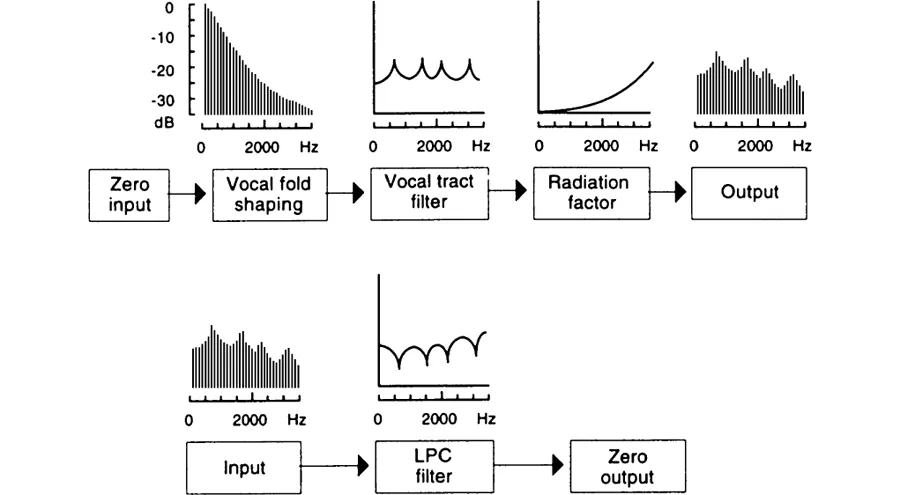
As we saw in chapter 7, we can describe many of the sounds of speech in terms of a source-filter theory, summarized in figure 7.7, reproduced here as the top half of figure 11.1. We have added to the original figure 7.7, in that we have imagined that we began with a zero input which then became shaped so that it was equivalent to the vocal cord source, a set of pulses with a particular shape. Of course, if there really were a zero input and no generator within the system, there would be no output. The notion of a zero input is simply a convenient way of emphasizing that the vocal cord pulses are part of the production system. From there the diagram goes on as before, with the sound produced at the glottis being filtered by the vocal tract, and then becoming a source of sound radiating out from the lips. The sound wave that is produced is represented by its spectrum on the right at the top of figure 11.1.

Fig. 11.1. A source-filter view of speech synthesis compared with LPC analysis.

The basic notion of an LPC analysis is shown in the lower part of the figure. It can be regarded as the reverse of the process of speech production. In this analysis scheme, the input is a speech wave (represented here by its spectrum), which is passed through a filter that is the inverse of this spectrum and that will produce as close to a zero output as possible. There is a major difference between the two systems, apart from the fact that one is an account of speech synthesis and the other a system for speech analysis. In the LPC approach the spectral shaping characteristics of the glottal source and of the lip radiation are incorporated into the same filter as that representing the characteristics of the vocal tract. Consequently the LPC filter is not exactly the same as the vocal tract filter. It does, however, have the same general shape; and the important similarity between the two systems is that in each case the principal activity is one of filtering a waveform. Accordingly, we will begin this account of LPC analysis by considering filters in digital terms.

Digital Filters

The characteristics of a filter are usually expressed in spectral terms. In chapters 5 and 6, when we first discussed filters, we did this by considering an input wave and then stating the center frequency and the bandwidth of the spectrum that the filter would pass. But in digital speech processing, it is not a wave that serves as input to the filter; it is a set of samples representing the amplitudes at discrete moments in time. We must therefore consider how the characteristics of a filter can be specified as an action performed on these points.

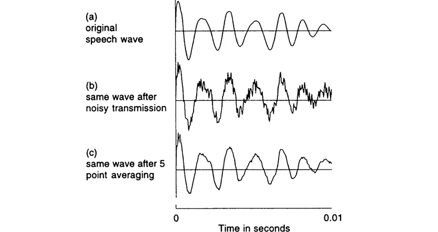
One example of such a specification is that for a moving average (MA) filter, which is a filter in which each point is replaced by the average of itself and the points around it. Consider the wave in figure 11.2(a). If this sound is transmitted through a noisy channel, such as a bad telephone line, it will have added random noise, as shown in figure 11.2(b). We can remove some of this noise by passing the wave through a filter that replaces every point by the mean of the point itself and a number of points on either side, thus taking a moving average. In this way we can recover something more like the original wave, although still with several irregularities, as shown in figure 11.2(c).

A more detailed look at this process is given in figure 11.3, which shows the individual points in a part of the noisy wave in figure 11.2(b), and the points after passing them through a filter which replaces every point by the mean of that point and the two points before it and the two points after it. In this particular example we are considering sets of five points. Instead of a five-point moving average, we could have taken a larger or a smaller number of points into account, thus producing more or less smoothing of the input wave.

Fig. 11.2. (a) Part of a speech wave; (b) the same wave after it has been passed through a nois...