Tunnelling in Molecules

Nuclear Quantum Effects from Bio to Physical Chemistry

Johannes Kästner, Sebastian Kozuch

• Publisher: Royal Society of Chemistry
• Year: 2020
• Print ISBN: 9781788018708
• eBook ISBN: 9781839160387
• Edition: 1
• Topic: Physical Sciences
• Subtopic: Physical & Theoretical Chemistry

Quantum tunnelling is one of the strangest phenomena in chemistry, where we see the wave nature of atoms acting in "impossible" ways. By letting molecules pass through the kinetic barrier instead of over it, this effect can lead to chemical reactions even close to the absolute zero, to atypical spectroscopic observations, to bizarre selectivity, or to colossal isotopic effects. Quantum mechanical tunnelling observations might be infrequent in chemistry, but it permeates through all its disciplines producing remarkable chemical outcomes. For that reason, the 21st century has seen a great increase in theoretical and experimental findings involving molecular tunnelling effects, as well as in novel techniques that permit their accurate predictions and analysis.

Including experimental, computational and theoretical chapters, from the physical and organic to the biochemistry fields, from the applied to the academic arenas, this new book provides a broad and conceptual perspective on tunnelling reactions and how to study them. Quantum Tunnelling in Molecules is the obligatory stop for both the specialist and those new to this world.

CHAPTER 1

Direct Observation of Tunnelling Reactions by Matrix Isolation Spectroscopy

CLÁUDIO M. NUNES,*^a IGOR REVA*^a AND RUI FAUSTO*^a,b

^a University of Coimbra, CQC, Department of Chemistry, 3004-535 Coimbra, Portugal

^b Department of Chemistry, King Fahd University of Petroleum and Minerals, 31261 Dhahran, Saudi Arabia

*Emails: [email protected]; [email protected]; [email protected]

1.1 Introduction

The theoretical foundations for nuclei and electron tunnelling were put forward by Hund,¹ Wigner,² Bell,³ and others,^4,5 following the establishment of quantum mechanics. A more generalized treatment of tunnelling in chemistry appeared almost half a century afterwards in the seminal Bell's monography “The Tunnel Effect in Chemistry”.^6,7 Indeed, as addressed in several other chapters of this book, theoretical methodologies to treat quantum mechanical tunnelling (QMT) in chemical reactions are still being developed nowadays. In this chapter, QMT in chemistry will be addressed from a more experimental perspective, taking advantage of the conditions typical of a matrix isolation experiment, which allow for direct observation of tunnelling driven processes by steady-state spectroscopic methods.

A simple and common way to portray tunnelling, although not particularly accurate,⁸ is to consider it as a phenomenon that arises from the wave–particle duality. If in a chemical reaction the moving distance of a nucleus is comparable to its de Broglie wavelength, then there is a non-negligible probability of finding the nucleus on the other side of the reaction barrier, even if the system does not possess enough thermal energy to surmount the barrier. It means that nuclei are able to penetrate through reaction barriers. Of course, such unexpected behavior is framed on a classic perspective, in which all atoms involved in a chemical transformation are assumed to behave as hard spheres.

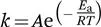
According to the classic transition state theory (TST), reactants must acquire enough energy to overcome a barrier in order to give rise to products.^9–11 Statistically, as temperature increases, more molecules will have enough energy to traverse the barrier, so that the reaction rate typically increases proportionally. Such temperature dependence of reaction rates was empirically established by Arrhenius in his well-known equation [eqn (1.1)], long before the development of the TST.^11,12

(1.1)

In eqn (1.1), A is a pre-exponential constant, E_a the activation energy (J mol⁻¹), R the universal gas constant (8.314 J mol⁻¹ K⁻¹), and T (K) is the absolute temperature.

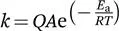
However, deviations from the Arrhenius typical behavior can take place if tunnelling occurs simultaneously with the classic passage over the barrier. In these cases, the QMT contribution to the reaction rate can be incorporated using a tunnelling correction factor Q in the kinetic models, as it is, for instance, shown in eqn (1.2).^6,11,13

(1.2)

The tunnelling correction factor Q takes into account the tunnelling permeability through the barrier, which depends on the mass of the tunnelling particle, as well as on the barrier height and width.^6,13

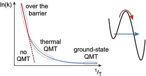
The existence of QMT contribution to a chemical reaction is typically detected indirectly by the observation of non-linear Arrhenius plots or abnormal kinetic isotope effects.^14–18 The temperature dependence of k in eqn (1.1) is given by the exponential factor, exp(−E_a/RT). Consequently, a plot of ln(k) against 1/T results in a straight line (see Figure 1.1). Its slope is −E_a/R. For historic reasons, such plots are referred to as Arrhenius plots. On the other hand, contrary to the classical over-the-barrier thermal process, tunnelling rates are approximately independent of the temperature. For a low enough temperature, when the system is in its ground vibrational state, the overall reaction rate is dominated by tunnelling and, consequently, temperature independent (see Figure 1.1).

Figure 1.1 Logarithm of the rate constant plotted versus the inverse temperature (Arrhenius plot). The classical (thermal) over-the-barrier reaction results in a straight line. The rate becomes constant at low temperature when ground-state quantum-mechanical tunnelling (QMT) dominates. Adapted from ref. 15 with permission from the Royal Society of Chemistry.

Working at low temperatures is in fact a very convenient way to search for evidence of tunnelling in chemical reactions. At cryogenic temperatures (e.g., 3–10 K), thermally activated rates become negligible for systems having barriers as low as ∼4 kJ mol⁻¹ (∼1 kcal mol⁻¹), so the occurrence of a chemical transformation can only be due to a “pure” tunnelling reaction.^14–18 If such tunnelling transformations span from seconds to days, they can be directly observed and monitored using stationary-state spectroscopy methods. Indeed, particularly during the last decade, direct spectroscopic evidence of a variety of tunnelling-driven reactions has been reported using the low-temperature matrix isolation technique coupled to infrared spectroscopy. These observations have contributed significantly to a better understanding of QMT and its role in chemistry.¹⁹

In this chapter, we will address some representative cases of tunnelling-driven chemical processes, from conformational isomerizations to H-atom and heavy-atom bond-breaking/bond-forming reactions occurring in organic molecules under matrix isolation conditions. Examples of tunnelling reactions at cryogenic temperatures taking place in other than matrix isolation conditions are outside the scope of this chapter.

1.2 Description of Simple Mathematic Models for Tunnelling Computations

The present chapter is not concerned with the theory of tunnelling. There are several recent reviews on the topic.^18,20–22 Here, we shall recall that any occurrence of a tunnelling reaction must always face a barrier to overcome. This section will present simple formulas for the probabilities of tunnelling through two barriers of different shapes.

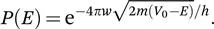
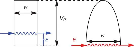
In a recent review,²² Borden presents the formula for the energy-dependent probability P(E), of a particle with mass m, tunnelling through a rectangular barrier of width w that is V₀−E higher than the energy of the particle (see Figure 1.2, left):

(1.3)

Figure 1.2 Left: tunnelling through a rectangular barrier of width w, at an energy V₀−E below the top of the barrier. Right: tunnelling through a parabolic barrier of width w, at an energy V₀−E below the top of the barrier.

A more realistic barrier shape is that of the inverted parabola (as in Figure 1.2, right). The approximate solutions for the equations describing the tunnelling of a particle through a parabolic barrier were independently devised by Wentzel, Kramers, and Brillouin in 1926.^23–25 As it is noted by Borden,²² “what has become known as the WKB approximate solution^23–25to the calculation of the probability of tunnelling through a parabolic barrier should really be known as the JWKB approximate solution”,²² because “earlier Jeffreys²⁶had published the mathematics necessary to obtain approximate solutions to differ...

Table of contents

• Cover
• Title
• Copyright
• Preface
• Contents
• Chapter 1 Direct Observation of Tunnelling Reactions by Matrix Isolation Spectroscopy
• Chapter 2 Tunnelling Instability in Molecular Systems. An Exercise in Computational Chemistry Prediction Power
• Chapter 3 Proton Tunnelling and Proton-coupled Electron Transfer in Biological Systems: Theory and Experimental Analysis
• Chapter 4 From Tunnelling Control to Controlling Tunnelling
• Chapter 5 From Nuclear Fluxes During Tunnelling to Electronic Fluxes During Charge Migration
• Chapter 6 Tunnelling and Parity Violation in Chiral and Achiral Molecules: Theory and High-resolution Spectroscopy
• Chapter 7 Instanton Theory to Calculate Tunnelling Rates and Tunnelling Splittings
• Chapter 8 Semiclassical Multidimensional Tunnelling Calculations
• Chapter 9 The Calculation of Tunnelling Splittings Illustrated on Malonaldehyde
• Chapter 10 Quantum-dynamical Calculation of Rate Constants in Polyatomic Reactions Employing the Quantum Transition State Concept
• Chapter 11 Eigenstate Approaches for High Resolution Spectroscopy of Tunnelling in Small Molecular Systems
• Chapter 12 The Tunnelling Flight Time
• Subject Index