Basic Experimental Strategies and Data Analysis for Science and Engineering

John Lawson, John Erjavec

• Publisher: Chapman and Hall/CRC
• Year: 2016
• Print ISBN: 9781466512177
• eBook ISBN: 9781315356914
• Edition: 1
• Topic: Business
• Subtopic: Operations
• Index: Business

Every technical investigation involving trial-and-error experimentation embodies a strategy for deciding what experiments to perform, when to quit, and how to interpret the data. This handbook presents several statistically derived strategies which are more efficient than any intuitive approach and will get the investigator to their goal with the fewest experiments, give the greatest degree of reliability to their conclusions, and keep the risk of overlooking something of practical importance to a minimum.

Features:

• 
  
  

• Provides a comprehensive desk reference on experimental design that will be useful to practitioners without extensive statistical knowledge
• Features a review of the necessary statistical prerequisites
• Presents a set of tables that allow readers to quickly access various experimental designs
• Includes a roadmap for where and when to use various experimental design strategies
• Shows compelling examples of each method discussed
• Illustrates how to reproduce results using several popular software packages on a companion web site

Following the outlines and examples in this book should quickly allow a working professional or student to select the appropriate experimental design for a research problem at hand, follow the design to conduct the experiments, and analyze and interpret the resulting data.

John Lawson and John Erjavec have a combined 25 years of industrial experience and over 40 years of academic experience. They have taught this material to numerous practicing engineers and scientists as well as undergraduate and graduate students.

Chapter 1

Strategies for Experimentation with Multiple Factors

1.1 Introduction

Advancements in knowledge through the scientific method are obtained by iterating through three basic steps: conjecture, observation, and analysis. In the conjecture step, a theory or hypothesis is formulated to explain the causes for the behavior of the system or phenomenon under study. In the observation and analysis steps, data is collected and analyzed to confirm or contradict the consequences of the proposed theory or hypothesis. The value of statistical methods in the analysis and interpretation of research data is well understood. Articles in reputable journals justify their conclusions based on the level of statistical significance. Less understood is the vital role of statistical methods in the collection of data, especially in research studies aimed at establishing cause and effect links, or determining optimum operating conditions.

One of the statistical methods used in data collection is called the statistical design of experiments, or just design for short. In practice, using a good strategy for data collection (i.e., a good design) is even more important than a statistical analysis of the results. That is because it is difficult, if not impossible, to remedy the problems inherent in a less than optimal data collection strategy, even with the most sophisticated statistical analysis. As the old adage goes: “You can’t make a silk purse out of a sow’s ear.” On the other hand, it is difficult (but not impossible) to mangle the interpretation of a well-designed set of experiments.

These two tools—statistical design and statistical analysis—are used very fruitfully in finding empirical solutions to industrial problems and basic research. The areas of application include research, product design, process design, production troubleshooting, and production optimization. The response or objective in a research or industrial study is usually a function of many interrelated factors, so solving these problems is typically not straightforward. There are two broad categories of approaches to these problems: 1) finding solutions by invoking known theory or facts, including experience with similar problems or situations, and 2) finding solutions through trial and error or experimentation. Statistical design and analysis methods are very useful for the second approach, and they are much more effective than any traditional, nonstatistical method.

In this book we present some well-proven experimental design plans to (1) screen which variables (from a multitude of possible factors) have important effects, (2) determine optimum operating conditions with respect to a few important variables, and (3) describe variability in research data. In each case we illustrate the corresponding methods for analyzing the resulting data. The plans are tabulated in appendices to the book, and available for download from the website for this book. Most of the analysis can be conducted using spreadsheet software like Microsoft Excel^© or Libre Office Calc^©.

1.2 Some Definitions

Before beginning a discussion of statistical design and statistical analysis, it is important to ensure that we are all speaking the same language. So let us define several of the terms that we will use frequently.

• Experiment (also called a Run)—an action in which the experimenter changes at least one of the factors being studied and then observes the effect of his/her action(s). Note that the passive collection of historical data is not experimentation.

• Experimental Unit—the item under study upon which something is changed. In a chemical experiment it could be a batch of material that is made under certain conditions. The conditions would be changed from one unit (batch) to the next. In a mechanical experiment it could be a prototype model or a fabricated part.

• Factor (also called an Independent Variable and denoted by the symbol, X) —one of the variables under study which is being deliberately controlled at or near some target value during any given experiment. Its target value is being changed in some systematic way from run to run in order to determine what effect it has on the response(s).

• Background Variable (also called a Lurking Variable)—a variable of which the experimenter is unaware or cannot control, and which could have an effect on the outcome of an experiment. The effects of these lurking variables should be given a chance to “balance out” in the experimental pattern. Later in this book we will discuss techniques (specifically randomization and blocking) to help ensure that goal.

• Response (also called a Dependent Variable and denoted by the symbol, Y)—a characteristic of the experimental unit which is measured during and/or after each run. The value of the response depends on the settings of the factors or independent variables (X’s).

• Effect— is the expected change in the response that results when the value of a factor is changed.

• Experimental Design (also called Experimental Pattern)—the collection of experiments to be run. We have also been calling this the experimental strategy.

• Experimental Error—the difference between any given observed response, Y, and the long run average (or “true” value of Y) at a particular set of experimental conditions. This error is a fact of life. There is variability (or imprecision) in all experiments. The fact that it is called “error” should not be construed as meaning it is due to a blunder or mistake. Experimental errors may be broadly classified into two types: bias errors and random errors. A bias error tends to remain constant or follow a consistent pattern over the course of the experimental design. Random errors, on the other hand, change value from one experiment to the next with an average value of zero. The principal tools for dealing with bias errors are blocking and randomization (of the order of the experimental runs). The tool to deal with random error is replication. All of these will be discussed in detail later.

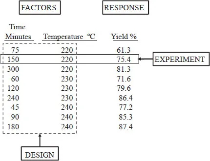
Some of the terms are illustrated in Figure 1.1. It is a study of a chemical reaction (A + B → P) consisting of nine runs to determine the effects of two factors (time and temperature) on one response (yield). One run (or experiment) consists of setting the temperature, allowing the reaction to go on for the specified time, and then measuring the yield. The design is the collection of all runs that will be (or were) made.

FIGURE 1.1: Example of an Experimental Study with Terminology Illustrated

1.3 Classical Versus Statistical Approaches to Experimentation

A typical strategy for a research study used by someone unfamiliar with statistical plans is the one-at-a-time design. In this approach, a solution is sought by methodically varying one factor at a time (usually performing numerous experiments at many different values of that factor), while all other factors are held constant at some reasonable values. This process is then repeated for each of the other factors, in turn. One-at-a-time is a very time-consuming strategy, but it has at least two good points. First, it is simple, which is not a virtue to be sneezed at. And second, it lends itself easily to a graphical display of results. People think best in terms of pictures, so this is also a very important benefit.

Unfortunately, one-at-a-time usually results in a less than optimal solution to a problem, despite the extra work and consequent expense. The reason is that one-at-a-time experimentation is only a good strategy under what we consider to be unusual circumstances. These unusual circumstances would include the following characteristics: (1) the response is a complicated function of the factors, X’s (perhaps multimodal), which requires many levels of each X to elucidate, (2) the response relationship with the factors dominates the experimental error and will be recognized in the presence of this error, (3) the effect of the factor being studied (and therefore its optimum value) is not changed by the level of any of the other factors. That is, the one-at-a time strategy works only if the effects are strictly additive, and the effect of one factor does not depend on others. As was just stated, but worth repeating, these circumstances do not typically exist in the real world, and so one-at-a-time ends up being an exceedingly poor approach to problem solving.

The assumptions made by statistical designs represent a more typical set of circumstances. They are: (1) within the experimental region, the response is smooth with, at most, some curvature but no sharp kinks or inflection points, (2) experimental error is always present to ”muddy the water” of experimental results, and (3) the effect of one factor can depend on the level of one or more of the other factors. In other words, there may be dependencies or interactions between factor’s effects. If these assumptions hold, the classical one-at-a-time approach could do very badly. If the first assumption holds, one-at-a-time would require many more experiments to do the same job, because fewer levels of a factor are needed to fit a smooth response than to fit a complicated one. If the second and third assumption hold, one-at-a-time could lead to completely misleading conclusions.

For example, if we try to find the optimal time and temperature for the yield of a chemi...

Table of contents

• Cover
• Half Title
• Title Page
• Copyright Page
• Dedication
• Table of Contents
• List of Figures
• List of Tables
• Preface
• Author Bios
• 1 Strategies for Experimentation with Multiple Factors
• 2 Statistics and Probability
• 3 Basic Two-Level Factorial Experiments
• 4 Additional Tools for Two-Level Factorials
• 5 General Factorial Experiments and ANOVA
• 6 Variance Component Studies
• 7 Screening Designs
• 8 Regression Analysis
• 9 Response Surface Designs
• 10 Response Surface Model Fitting
• 11 Sequential Experimentation
• 12 Mixture Experiments
• 13 Practical Suggestions for Successful Experimentation
• Appendix A
• Appendix B
• Check Figures for Selected Exercises
• Bibliography
• Index