![]()
CHAPTER 1
Introduction
The discipline of operations research was born out of the need to solve military problems during World War II. In one story, the air force was using the bullet holes on the airplanes used in combat duty to decide where to put extra armor plating. They thought they were approaching the problem in a scientific way until someone pointed out that they were collecting the bullet hole data from the planes that returned safely from their sorties.
1.1 What in the World Is a Stochastic Process?
Consider a system that evolves randomly in time, for example, the stock market index, the inventory in a warehouse, the queue of customers at a service station, water level in a reservoir, the state of a machines in a factory, etc.
Suppose we observe this system at discrete time points n = 0, 1, 2, …, say, every hour, every day, every week, etc. Let Xn be the state of the system at time n. For example, Xn can be the Dow-Jones index at the end of the n-th working day; the number of unsold cars on a dealer’s lot at the beginning of day n; the intensity of the n-th earthquake (measured on the Richter scale) to hit the continental United States in this century; or the number of robberies in a city on day n, to name a few. We say that {Xn, n ≥ 0} is a discrete-time stochastic process describing the system.
If the system is observed continuously in time, with X(t) being its state at time t, then it is described by a continuous time stochastic process {X(t), t ≥ 0}. For example, X(t) may represent the number of failed machines in a machine shop at time t, the position of a hurricane at time t, or the amount of money in a bank account at time t, etc.
More formally, a stochastic process is a collection of random variables {X(τ), τ ∈ T}, indexed by the parameter τ taking values in the parameter set T. The random variables take values in the set S, called the state-space of the stochastic process. In many applications the parameter τ represents time, but it can represent any index. Throughout this book we shall encounter two cases:
1. T = {0, 1, 2, …}. In this case we write {Xn, n ≥ 0} instead of {X(τ), τ ∈ T}.
2. T = [0, ∞). In this case we write {X(t), t ≥ 0} instead of {X(τ), τ ∈ T}.
Also, we shall almost always encounter S ⊆ {0, 1, 2, …} or S ⊆ (−∞, ∞). We shall refer to the former case as the discrete state-space case, and the latter case as the continuous state-space case.
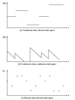
Let {X(τ), τ ∈ T} be a stochastic process with state-space S, and let x: T → S be a function. One can think of {x(τ), τ ∈ T} as a possible evolution (trajectory) of {X(τ), τ ∈ T}. The functions x are called the sample paths of the stochastic process. Figure 1.1 shows typical sample paths of stochastic processes. Since the stochastic process follows one of the sample paths in a random fashion, it is sometimes called a random function. In general, the set of all possible sample paths, called the sample space of the stochastic process, is uncountable. This can be true even in the case of a discrete time stochastic process with finite state-space. One of the aims of the study of the stochastic processes is to understand the behavior of the random sample paths that the system follows, with the ultimate aim of prediction and control of the future of the system.
Figure 1.1 Typical sample paths of stochastic processes.
Stochastic processes are used in epidemiology, biology, demography, health care systems, polymer science, physics, telecommunication networks, economics, finance, marketing, and social networks, to name a few areas. A vast literature exists in each of these areas. Our applications will generally come from queueing theory, inventory systems, supply chains, manufacturing, health care systems, computer and communication networks, reliability, warranty management, mathematical finance, and statistics. We illustrate a few such applications in the example below. Although most of the applications seem to involve continuous time stochastic process, they can easily be converted into discrete time stochastic processes by simply assuming that the system in question is observed at a discrete set of points, such as each hour, or each day, etc.
Example 1.1 Examples of Stochastic Processes in Real Life
Queues. Let X(t) be the number of customers waiting for service in a service facility such as an outpatient clinic. {X(t), t ≥ 0} is a continuous time stochastic process with state-space S = {0, 1, 2, …}.
Inventories. Let X(t) be the number of automobiles in the parking lot of a dealership available for sale at time t, and Y(t) be the number of automobiles on order (the customers have paid a deposit for them and are now waiting for delivery) at the dealership at time t. Both {X(t), t ≥ 0} and {Y(t), t ≥ 0} are continuous time stochastic processes with state-space S = {0, 1, 2, …}.
Supply Chains. Consider a supply chain of c...